scipy.special.sici#

scipy.special.sici(x, out=None) = <ufunc 'sici'>#

正弦和餘弦積分。

正弦積分為

\[\int_0^x \frac{\sin{t}}{t}dt\]

而餘弦積分為

\[\gamma + \log(x) + \int_0^x \frac{\cos{t} - 1}{t}dt\]

其中 \(\gamma\) 是歐拉常數，而 \(\log\) 是對數的主分支 [1]。

參數:

xarray_like: 計算正弦和餘弦積分的實數或複數點。
outtuple of ndarray, optional: 函數結果的可選輸出陣列

返回:

siscalar or ndarray: 在 x 處的正弦積分
ciscalar or ndarray: 在 x 處的餘弦積分

參見

shichi: 雙曲正弦和餘弦積分。
exp1: 指數積分 E1。
expi: 指數積分 Ei。

註解

對於實數參數且 x < 0，ci 是餘弦積分的實部。對於這些點，ci(x) 和 ci(x + 0j) 相差 1j*pi 倍。

對於實數參數，此函數透過呼叫 Cephes 的 [2] sici 常式來計算。對於複數參數，此演算法基於 Mpmath 的 [3] si 和 ci 常式。

參考文獻

[1] (1,2)

Milton Abramowitz and Irene A. Stegun, eds. Handbook of Mathematical Functions with Formulas, Graphs, and Mathematical Tables. New York: Dover, 1972. (See Section 5.2.)

[2]

Cephes Mathematical Functions Library, http://www.netlib.org/cephes/

[3]

Fredrik Johansson and others. “mpmath: a Python library for arbitrary-precision floating-point arithmetic” (Version 0.19) http://mpmath.org/

範例

>>> import numpy as np
>>> import matplotlib.pyplot as plt
>>> from scipy.special import sici, exp1

sici 接受實數或複數輸入

>>> sici(2.5)
(1.7785201734438267, 0.2858711963653835)
>>> sici(2.5 + 3j)
((4.505735874563953+0.06863305018999577j),
(0.0793644206906966-2.935510262937543j))

對於右半平面的 z，正弦和餘弦積分與指數積分 E1（在 SciPy 中實作為 scipy.special.exp1）相關，關係如下

Si(z) = (E1(i*z) - E1(-i*z))/2i + pi/2
Ci(z) = -(E1(i*z) + E1(-i*z))/2

參見 [1]（方程式 5.2.21 和 5.2.23）。

我們可以驗證這些關係

>>> z = 2 - 3j
>>> sici(z)
((4.54751388956229-1.3991965806460565j),
(1.408292501520851+2.9836177420296055j))

>>> (exp1(1j*z) - exp1(-1j*z))/2j + np.pi/2  # Same as sine integral
(4.54751388956229-1.3991965806460565j)

>>> -(exp1(1j*z) + exp1(-1j*z))/2            # Same as cosine integral
(1.408292501520851+2.9836177420296055j)

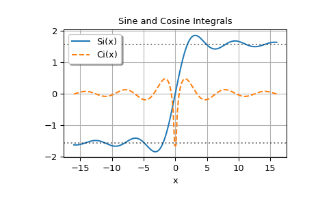
繪製在實軸上評估的函數；虛線水平線位於 pi/2 和 -pi/2

>>> x = np.linspace(-16, 16, 150)
>>> si, ci = sici(x)

>>> fig, ax = plt.subplots()
>>> ax.plot(x, si, label='Si(x)')
>>> ax.plot(x, ci, '--', label='Ci(x)')
>>> ax.legend(shadow=True, framealpha=1, loc='upper left')
>>> ax.set_xlabel('x')
>>> ax.set_title('Sine and Cosine Integrals')
>>> ax.axhline(np.pi/2, linestyle=':', alpha=0.5, color='k')
>>> ax.axhline(-np.pi/2, linestyle=':', alpha=0.5, color='k')
>>> ax.grid(True)
>>> plt.show()