scipy.special.shichi#

scipy.special.shichi(x, out=None) = <ufunc 'shichi'>#

雙曲正弦和餘弦積分。

雙曲正弦積分為

\[\int_0^x \frac{\sinh{t}}{t}dt\]

而雙曲餘弦積分為

\[\gamma + \log(x) + \int_0^x \frac{\cosh{t} - 1}{t} dt\]

其中 \(\gamma\) 是歐拉常數，而 \(\log\) 是對數函數的主分支 [1]。

參數:

xarray_like: 計算雙曲正弦和餘弦積分的實數或複數點。
outndarray 元組，選用: 函數結果的選用輸出陣列

回傳:

si純量或 ndarray: 在 x 的雙曲正弦積分
ci純量或 ndarray: 在 x 的雙曲餘弦積分

參見

sici: 正弦和餘弦積分。
exp1: 指數積分 E1。
expi: 指數積分 Ei。

註解

對於 x < 0 的實數參數，chi 是雙曲餘弦積分的實部。對於這些點，chi(x) 和 chi(x + 0j) 相差 1j*pi 倍。

對於實數參數，此函數透過呼叫 Cephes 的 [2] shichi 常式來計算。對於複數參數，此演算法基於 Mpmath 的 [3] shi 和 chi 常式。

參考文獻

[1]

Milton Abramowitz 和 Irene A. Stegun，編輯。《Handbook of Mathematical Functions with Formulas, Graphs, and Mathematical Tables》。紐約：Dover，1972。(參見第 5.2 節。)

[2]

Cephes 數學函數庫，http://www.netlib.org/cephes/

[3]

Fredrik Johansson 及其他作者。「mpmath：用於任意精度浮點運算的 Python 庫」(版本 0.19) http://mpmath.org/

範例

>>> import numpy as np
>>> import matplotlib.pyplot as plt
>>> from scipy.special import shichi, sici

shichi 接受實數或複數輸入

>>> shichi(0.5)
(0.5069967498196671, -0.05277684495649357)
>>> shichi(0.5 + 2.5j)
((0.11772029666668238+1.831091777729851j),
 (0.29912435887648825+1.7395351121166562j))

雙曲正弦和餘弦積分 Shi(z) 和 Chi(z) 與正弦和餘弦積分 Si(z) 和 Ci(z) 的關係為

Shi(z) = -i*Si(i*z)
Chi(z) = Ci(-i*z) + i*pi/2

>>> z = 0.25 + 5j
>>> shi, chi = shichi(z)
>>> shi, -1j*sici(1j*z)[0]            # Should be the same.
((-0.04834719325101729+1.5469354086921228j),
 (-0.04834719325101729+1.5469354086921228j))
>>> chi, sici(-1j*z)[1] + 1j*np.pi/2  # Should be the same.
((-0.19568708973868087+1.556276312103824j),
 (-0.19568708973868087+1.556276312103824j))

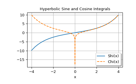
繪製在實軸上評估的函數

>>> xp = np.geomspace(1e-8, 4.0, 250)
>>> x = np.concatenate((-xp[::-1], xp))
>>> shi, chi = shichi(x)

>>> fig, ax = plt.subplots()
>>> ax.plot(x, shi, label='Shi(x)')
>>> ax.plot(x, chi, '--', label='Chi(x)')
>>> ax.set_xlabel('x')
>>> ax.set_title('Hyperbolic Sine and Cosine Integrals')
>>> ax.legend(shadow=True, framealpha=1, loc='lower right')
>>> ax.grid(True)
>>> plt.show()

../../_images/scipy-special-shichi-1.png