iirfilter#
- scipy.signal.iirfilter(N, Wn, rp=None, rs=None, btype='band', analog=False, ftype='butter', output='ba', fs=None)[原始碼]#
給定階數和臨界點的 IIR 數位和類比濾波器設計。
設計 N 階數位或類比濾波器,並傳回濾波器係數。
- 參數:
- Nint
濾波器的階數。
- Wnarray_like
純量或長度為 2 的序列,給定臨界頻率。
對於數位濾波器,Wn 的單位與 fs 相同。預設情況下,fs 為 2 半週期/樣本,因此這些值已標準化為 0 到 1,其中 1 為奈奎斯特頻率。(Wn 的單位因此為半週期/樣本。)
對於類比濾波器,Wn 為角頻率(例如,rad/s)。
當 Wn 是長度為 2 的序列時,
Wn[0]必須小於Wn[1]。- rpfloat, optional
對於 Chebyshev 和橢圓濾波器,提供通帶中的最大漣波。(分貝)
- rsfloat, optional
對於 Chebyshev 和橢圓濾波器,提供阻帶中的最小衰減。(分貝)
- btype{‘bandpass’, ‘lowpass’, ‘highpass’, ‘bandstop’}, optional
濾波器的類型。預設值為 ‘bandpass’。
- analogbool, optional
為 True 時,傳回類比濾波器,否則傳回數位濾波器。
- ftypestr, optional
要設計的 IIR 濾波器類型
Butterworth : ‘butter’
Chebyshev I : ‘cheby1’
Chebyshev II : ‘cheby2’
Cauer/elliptic: ‘ellip’
Bessel/Thomson: ‘bessel’
- output{‘ba’, ‘zpk’, ‘sos’}, optional
輸出的濾波器形式
二階區段(建議):‘sos’
分子/分母(預設):‘ba’
極點-零點:‘zpk’
一般而言,建議使用二階區段(‘sos’)形式,因為推斷分子/分母形式(‘ba’)的係數會受到數值不穩定性的影響。 由於向後相容性的原因,預設形式是分子/分母形式(‘ba’),其中 ‘ba’ 中的 ‘b’ 和 ‘a’ 指的是常用的係數名稱。
注意:使用二階區段形式(‘sos’)有時會產生額外的計算成本:因此,對於數據密集型用例,也建議研究分子/分母形式(‘ba’)。
- fsfloat, optional
數位系統的取樣頻率。
在 1.2.0 版本中新增。
- 傳回值:
- b, andarray, ndarray
IIR 濾波器的分子 (b) 和分母 (a) 多項式。僅在
output='ba'時傳回。- z, p, kndarray, ndarray, float
IIR 濾波器傳遞函數的零點、極點和系統增益。僅在
output='zpk'時傳回。- sosndarray
IIR 濾波器的二階區段表示法。僅在
output='sos'時傳回。
另請參閱
筆記
'sos'輸出參數是在 0.16.0 版本中新增的。範例
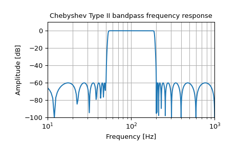
產生一個從 50 Hz 到 200 Hz 的 17 階 Chebyshev II 類比帶通濾波器,並繪製頻率響應
>>> import numpy as np
>>> from scipy import signal
>>> import matplotlib.pyplot as plt
>>> b, a = signal.iirfilter(17, [2*np.pi*50, 2*np.pi*200], rs=60,
...                         btype='band', analog=True, ftype='cheby2')
>>> w, h = signal.freqs(b, a, 1000)
>>> fig = plt.figure()
>>> ax = fig.add_subplot(1, 1, 1)
>>> ax.semilogx(w / (2*np.pi), 20 * np.log10(np.maximum(abs(h), 1e-5)))
>>> ax.set_title('Chebyshev Type II bandpass frequency response')
>>> ax.set_xlabel('Frequency [Hz]')
>>> ax.set_ylabel('Amplitude [dB]')
>>> ax.axis((10, 1000, -100, 10))
>>> ax.grid(which='both', axis='both')
>>> plt.show()
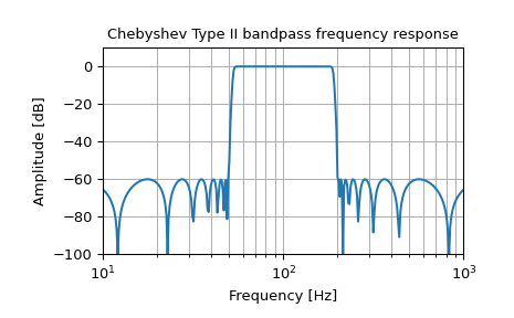
在取樣率為 2000 Hz 的系統中,建立具有相同屬性的數位濾波器,並繪製頻率響應。(需要二階區段實作以確保此階數濾波器的穩定性)
>>> sos = signal.iirfilter(17, [50, 200], rs=60, btype='band',
...                        analog=False, ftype='cheby2', fs=2000,
...                        output='sos')
>>> w, h = signal.freqz_sos(sos, 2000, fs=2000)
>>> fig = plt.figure()
>>> ax = fig.add_subplot(1, 1, 1)
>>> ax.semilogx(w, 20 * np.log10(np.maximum(abs(h), 1e-5)))
>>> ax.set_title('Chebyshev Type II bandpass frequency response')
>>> ax.set_xlabel('Frequency [Hz]')
>>> ax.set_ylabel('Amplitude [dB]')
>>> ax.axis((10, 1000, -100, 10))
>>> ax.grid(which='both', axis='both')
>>> plt.show()