scipy.special.yn#

scipy.special.yn(n, x, out=None) = <ufunc 'yn'>#

整數階和實數自變數的第二類貝索函數。

參數：:

narray_like: 階數 (整數)。
xarray_like: 自變數 (浮點數)。
outndarray, optional: 函數結果的可選輸出陣列

回傳值：:

Y純量或 ndarray: 貝索函數 \(Y_n(x)\) 的值。

參見

yv: 適用於實數階和實數或複數自變數。
y0: 此函數針對階數 0 的更快實作
y1: 此函數針對階數 1 的更快實作

註解

Cephes [1] 常式 yn 的包裝函式。

此函數透過對 n 的正向遞迴進行評估，從 Cephes 常式 y0 和 y1 計算的值開始。如果 n = 0 或 1，則直接呼叫 y0 或 y1 的常式。

參考文獻

[1]

Cephes 數學函數庫，http://www.netlib.org/cephes/

範例

在一個點評估 0 階函數。

>>> from scipy.special import yn
>>> yn(0, 1.)
0.08825696421567697

在一個點評估不同階數的函數。

>>> yn(0, 1.), yn(1, 1.), yn(2, 1.)
(0.08825696421567697, -0.7812128213002888, -1.6506826068162546)

透過提供列表或 NumPy 陣列作為 v 參數的引數，可以在一次呼叫中執行不同階數的評估

>>> yn([0, 1, 2], 1.)
array([ 0.08825696, -0.78121282, -1.65068261])

透過為 z 提供陣列，在多個點評估 0 階函數。

>>> import numpy as np
>>> points = np.array([0.5, 3., 8.])
>>> yn(0, points)
array([-0.44451873,  0.37685001,  0.22352149])

如果 z 是陣列，則如果要在一次呼叫中計算不同的階數，則階數參數 v 必須可廣播到正確的形狀。若要計算 1D 陣列的階數 0 和 1

>>> orders = np.array([[0], [1]])
>>> orders.shape
(2, 1)

>>> yn(orders, points)
array([[-0.44451873,  0.37685001,  0.22352149],
       [-1.47147239,  0.32467442, -0.15806046]])

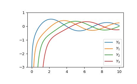
繪製從 0 到 10 的階數 0 到 3 的函數圖。

>>> import matplotlib.pyplot as plt
>>> fig, ax = plt.subplots()
>>> x = np.linspace(0., 10., 1000)
>>> for i in range(4):
...     ax.plot(x, yn(i, x), label=f'$Y_{i!r}$')
>>> ax.set_ylim(-3, 1)
>>> ax.legend()
>>> plt.show()