scipy.special.stdtrit#

scipy.special.stdtrit(df, p, out=None) = <ufunc 'stdtrit'>#

Student t 分佈的第 p 個分位數。

此函數是 Student t 分佈累積分布函數 (CDF) 的反函數，傳回 t 使得 stdtr(df, t) = p。

傳回引數 t 使得 stdtr(df, t) 等於 p。

參數:

dfarray_like: 自由度
parray_like: 機率
outndarray, optional: 函數結果的選用輸出陣列

傳回值:

tscalar or ndarray: t 的值，使得 stdtr(df, t) == p

參見

stdtr: Student t CDF
stdtridf: stdtr 相對於 df 的反函數
scipy.stats.t: Student t 分佈

註解

Student t 分佈也可以透過 scipy.stats.t 取得。直接呼叫 stdtrit 可以改善效能，相較於 scipy.stats.t 的 ppf 方法 (請參閱下方的最後一個範例)。

範例

stdtrit 代表 Student t 分佈 CDF 的反函數，而 Student t 分佈 CDF 可透過 stdtr 取得。在此，我們計算 df 在 x=1 的 CDF。stdtrit 接著會傳回 1，直到浮點誤差，給定相同的 df 值和計算出的 CDF 值。

>>> import numpy as np
>>> from scipy.special import stdtr, stdtrit
>>> import matplotlib.pyplot as plt
>>> df = 3
>>> x = 1
>>> cdf_value = stdtr(df, x)
>>> stdtrit(df, cdf_value)
0.9999999994418539

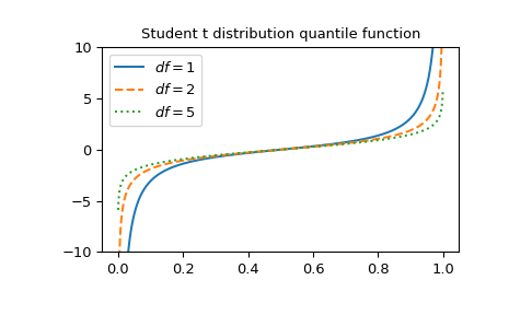
繪製三個不同自由度下的函數圖。

>>> x = np.linspace(0, 1, 1000)
>>> parameters = [(1, "solid"), (2, "dashed"), (5, "dotted")]
>>> fig, ax = plt.subplots()
>>> for (df, linestyle) in parameters:
...     ax.plot(x, stdtrit(df, x), ls=linestyle, label=f"$df={df}$")
>>> ax.legend()
>>> ax.set_ylim(-10, 10)
>>> ax.set_title("Student t distribution quantile function")
>>> plt.show()

../../_images/scipy-special-stdtrit-1_00_00.png

透過為 df 提供 NumPy 陣列或列表，可以同時計算多個自由度的函數

>>> stdtrit([1, 2, 3], 0.7)
array([0.72654253, 0.6172134 , 0.58438973])

透過為 df 和 p 提供形狀相容於廣播的陣列，可以同時計算多個點在多個不同自由度的函數。計算 3 個自由度下 4 個點的 stdtrit，產生形狀為 3x4 的陣列。

>>> dfs = np.array([[1], [2], [3]])
>>> p = np.array([0.2, 0.4, 0.7, 0.8])
>>> dfs.shape, p.shape
((3, 1), (4,))

>>> stdtrit(dfs, p)
array([[-1.37638192, -0.3249197 ,  0.72654253,  1.37638192],
       [-1.06066017, -0.28867513,  0.6172134 ,  1.06066017],
       [-0.97847231, -0.27667066,  0.58438973,  0.97847231]])

t 分佈也可以透過 scipy.stats.t 取得。直接呼叫 stdtrit 可能比呼叫 scipy.stats.t 的 ppf 方法快得多。為了獲得相同的結果，必須使用以下參數化：scipy.stats.t(df).ppf(x) = stdtrit(df, x)。

>>> from scipy.stats import t
>>> df, x = 3, 0.5
>>> stdtrit_result = stdtrit(df, x)  # this can be faster than below
>>> stats_result = t(df).ppf(x)
>>> stats_result == stdtrit_result  # test that results are equal
True