scipy.special.stdtr#

scipy.special.stdtr(df, t, out=None) = <ufunc 'stdtr'>#

學生 t 分佈累積分布函數

傳回積分

\[\frac{\Gamma((df+1)/2)}{\sqrt{\pi df} \Gamma(df/2)} \int_{-\infty}^t (1+x^2/df)^{-(df+1)/2}\, dx\]

參數:

dfarray_like: 自由度
tarray_like: 積分上限
outndarray, optional: 函數結果的可選輸出陣列

傳回值:

純量或 ndarray: 在 t 的學生 t CDF 值

參見

stdtridf: stdtr 相對於 df 的反函數
stdtrit: stdtr 相對於 t 的反函數
scipy.stats.t: 學生 t 分佈

註解

學生 t 分佈也可以使用 scipy.stats.t。直接呼叫 stdtr 可以比 scipy.stats.t 的 cdf 方法提高效能（請參閱下面的最後一個範例）。

範例

計算 df=3 在 t=1 的函數值。

>>> import numpy as np
>>> from scipy.special import stdtr
>>> import matplotlib.pyplot as plt
>>> stdtr(3, 1)
0.8044988905221148

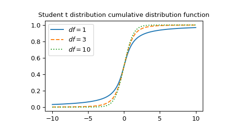
繪製三個不同自由度的函數圖。

>>> x = np.linspace(-10, 10, 1000)
>>> fig, ax = plt.subplots()
>>> parameters = [(1, "solid"), (3, "dashed"), (10, "dotted")]
>>> for (df, linestyle) in parameters:
...     ax.plot(x, stdtr(df, x), ls=linestyle, label=f"$df={df}$")
>>> ax.legend()
>>> ax.set_title("Student t distribution cumulative distribution function")
>>> plt.show()

../../_images/scipy-special-stdtr-1_00_00.png

透過為 df 提供 NumPy 陣列或列表，可以同時計算多個自由度的函數。

>>> stdtr([1, 2, 3], 1)
array([0.75      , 0.78867513, 0.80449889])

透過為 df 和 t 提供形狀相容於廣播的陣列，可以同時計算多個不同自由度下多個點的函數。計算 3 個自由度下 4 個點的 stdtr，產生形狀為 3x4 的陣列。

>>> dfs = np.array([[1], [2], [3]])
>>> t = np.array([2, 4, 6, 8])
>>> dfs.shape, t.shape
((3, 1), (4,))

>>> stdtr(dfs, t)
array([[0.85241638, 0.92202087, 0.94743154, 0.96041658],
       [0.90824829, 0.97140452, 0.98666426, 0.99236596],
       [0.93033702, 0.98599577, 0.99536364, 0.99796171]])

t 分佈也可以使用 scipy.stats.t。直接呼叫 stdtr 可能比呼叫 scipy.stats.t 的 cdf 方法快得多。若要獲得相同的結果，必須使用以下參數化：scipy.stats.t(df).cdf(x) = stdtr(df, x)。

>>> from scipy.stats import t
>>> df, x = 3, 1
>>> stdtr_result = stdtr(df, x)  # this can be faster than below
>>> stats_result = t(df).cdf(x)
>>> stats_result == stdtr_result  # test that results are equal
True