scipy.special.smirnov#
- scipy.special.smirnov(n, d, out=None) = <ufunc 'smirnov'>#
柯爾莫哥洛夫-斯米爾諾夫互補累積分布函數
返回精確的柯爾莫哥洛夫-斯米爾諾夫互補累積分布函數(又稱生存函數),用於檢驗經驗分布與理論分布之間是否相等的單邊檢定。它等於基於 n 個樣本的理論分布與經驗分布之間的最大差異大於 d 的機率。
- 參數:
- nint
樣本數
- dfloat array_like
經驗 CDF (ECDF) 與目標 CDF 之間的偏差。
- outndarray,可選
函數結果的可選輸出陣列
- 返回:
- 純量或 ndarray
smirnov(n, d) 的值,Prob(Dn+ >= d) (也適用於 Prob(Dn- >= d))
參見
smirnovi分布的反生存函數
scipy.stats.ksone以連續分布形式提供此功能
kolmogorov,kolmogi雙尾分布的函數
註記
smirnov由 stats.kstest 在應用柯爾莫哥洛夫-斯米爾諾夫適合度檢定時使用。由於歷史原因,此函數在 scpy.special 中公開,但要獲得最準確的 CDF/SF/PDF/PPF/ISF 計算,建議使用 stats.ksone 分布。範例
>>> import numpy as np
>>> from scipy.special import smirnov
>>> from scipy.stats import norm
顯示樣本數為 5 時,間隙至少為 0、0.5 和 1.0 的機率。
>>> smirnov(5, [0, 0.5, 1.0])
array([ 1.   ,  0.056,  0.   ])
將大小為 5 的樣本與 N(0, 1) 進行比較,N(0, 1) 是平均值為 0,標準差為 1 的標準常態分布。
x 是樣本。
>>> x = np.array([-1.392, -0.135, 0.114, 0.190, 1.82])
>>> target = norm(0, 1)
>>> cdfs = target.cdf(x)
>>> cdfs
array([0.0819612 , 0.44630594, 0.5453811 , 0.57534543, 0.9656205 ])
建構經驗累積分布函數和 K-S 統計量 (Dn+、Dn-、Dn)。
>>> n = len(x)
>>> ecdfs = np.arange(n+1, dtype=float)/n
>>> cols = np.column_stack([x, ecdfs[1:], cdfs, cdfs - ecdfs[:n],
...                        ecdfs[1:] - cdfs])
>>> with np.printoptions(precision=3):
...    print(cols)
[[-1.392  0.2    0.082  0.082  0.118]
 [-0.135  0.4    0.446  0.246 -0.046]
 [ 0.114  0.6    0.545  0.145  0.055]
 [ 0.19   0.8    0.575 -0.025  0.225]
 [ 1.82   1.     0.966  0.166  0.034]]
>>> gaps = cols[:, -2:]
>>> Dnpm = np.max(gaps, axis=0)
>>> print(f'Dn-={Dnpm[0]:f}, Dn+={Dnpm[1]:f}')
Dn-=0.246306, Dn+=0.224655
>>> probs = smirnov(n, Dnpm)
>>> print(f'For a sample of size {n} drawn from N(0, 1):',
...       f' Smirnov n={n}: Prob(Dn- >= {Dnpm[0]:f}) = {probs[0]:.4f}',
...       f' Smirnov n={n}: Prob(Dn+ >= {Dnpm[1]:f}) = {probs[1]:.4f}',
...       sep='\n')
For a sample of size 5 drawn from N(0, 1):
 Smirnov n=5: Prob(Dn- >= 0.246306) = 0.4711
 Smirnov n=5: Prob(Dn+ >= 0.224655) = 0.5245
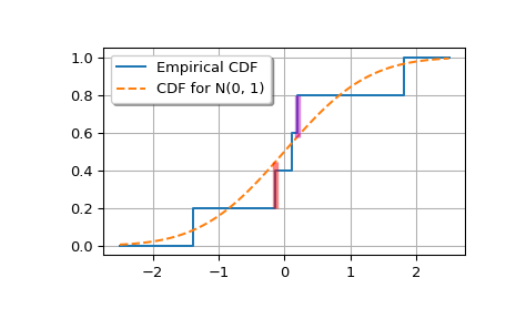
繪製經驗累積分布函數和標準常態累積分布函數。
>>> import matplotlib.pyplot as plt
>>> plt.step(np.concatenate(([-2.5], x, [2.5])),
...          np.concatenate((ecdfs, [1])),
...          where='post', label='Empirical CDF')
>>> xx = np.linspace(-2.5, 2.5, 100)
>>> plt.plot(xx, target.cdf(xx), '--', label='CDF for N(0, 1)')
新增標記 Dn+ 和 Dn- 的垂直線。
>>> iminus, iplus = np.argmax(gaps, axis=0)
>>> plt.vlines([x[iminus]], ecdfs[iminus], cdfs[iminus], color='r',
...            alpha=0.5, lw=4)
>>> plt.vlines([x[iplus]], cdfs[iplus], ecdfs[iplus+1], color='m',
...            alpha=0.5, lw=4)
>>> plt.grid(True)
>>> plt.legend(framealpha=1, shadow=True)
>>> plt.show()