scipy.special.kolmogorov

scipy.special.kolmogorov(y, out=None) = <ufunc 'kolmogorov'>

Kolmogorov 分佈的互補累積分布函數（生存函數）。

返回 Kolmogorov 極限分佈的互補累積分布函數（當 n 趨近於無限大時的 D_n*\sqrt(n)），用於檢驗經驗分布和理論分布之間是否相等的雙尾檢定。它等於（當 n->無限大時的極限）機率，即 sqrt(n) * max absolute deviation > y。

參數:

y浮點數 陣列型

經驗累積分布函數 (ECDF) 和目標累積分布函數 (CDF) 之間的絕對偏差，乘以 sqrt(n)。

outndarray，選填

用於函數結果的可選輸出陣列

回傳值:

純量或 ndarray

kolmogorov(y) 的值

另請參閱

kolmogi

分佈的反生存函數

scipy.stats.kstwobign

以連續分佈的形式提供功能

smirnov, smirnovi

用於單尾分佈的函數

註解

kolmogorov 被 stats.kstest 用於 Kolmogorov-Smirnov 適合度檢定。基於歷史原因，此函數在 scpy.special 中公開，但要獲得最準確的 CDF/SF/PDF/PPF/ISF 計算，建議使用 stats.kstwobign 分佈。

範例

在您的瀏覽器中試試看！

顯示間隙至少為 0、0.5 和 1.0 的機率。

>>> import numpy as np
>>> from scipy.special import kolmogorov
>>> from scipy.stats import kstwobign
>>> kolmogorov([0, 0.5, 1.0])
array([ 1.        ,  0.96394524,  0.26999967])

將從 Laplace(0, 1) 分佈中抽取的 1000 個樣本與目標分佈 Normal(0, 1) 分佈進行比較。

>>> from scipy.stats import norm, laplace
>>> rng = np.random.default_rng()
>>> n = 1000
>>> lap01 = laplace(0, 1)
>>> x = np.sort(lap01.rvs(n, random_state=rng))
>>> np.mean(x), np.std(x)
(-0.05841730131499543, 1.3968109101997568)

建構經驗累積分布函數 (Empirical CDF) 和 K-S 統計量 Dn。

>>> target = norm(0,1)  # Normal mean 0, stddev 1
>>> cdfs = target.cdf(x)
>>> ecdfs = np.arange(n+1, dtype=float)/n
>>> gaps = np.column_stack([cdfs - ecdfs[:n], ecdfs[1:] - cdfs])
>>> Dn = np.max(gaps)
>>> Kn = np.sqrt(n) * Dn
>>> print('Dn=%f, sqrt(n)*Dn=%f' % (Dn, Kn))
Dn=0.043363, sqrt(n)*Dn=1.371265
>>> print(chr(10).join(['For a sample of size n drawn from a N(0, 1) distribution:',
...   ' the approximate Kolmogorov probability that sqrt(n)*Dn>=%f is %f' %
...    (Kn, kolmogorov(Kn)),
...   ' the approximate Kolmogorov probability that sqrt(n)*Dn<=%f is %f' %
...    (Kn, kstwobign.cdf(Kn))]))
For a sample of size n drawn from a N(0, 1) distribution:
 the approximate Kolmogorov probability that sqrt(n)*Dn>=1.371265 is 0.046533
 the approximate Kolmogorov probability that sqrt(n)*Dn<=1.371265 is 0.953467

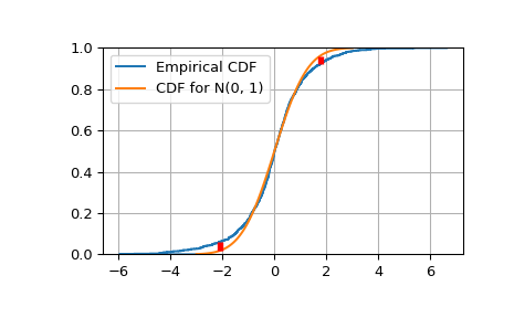
繪製經驗累積分布函數 (Empirical CDF) 對目標 N(0, 1) 累積分布函數 (CDF) 的圖。

>>> import matplotlib.pyplot as plt
>>> plt.step(np.concatenate([[-3], x]), ecdfs, where='post', label='Empirical CDF')
>>> x3 = np.linspace(-3, 3, 100)
>>> plt.plot(x3, target.cdf(x3), label='CDF for N(0, 1)')
>>> plt.ylim([0, 1]); plt.grid(True); plt.legend();
>>> # Add vertical lines marking Dn+ and Dn-
>>> iminus, iplus = np.argmax(gaps, axis=0)
>>> plt.vlines([x[iminus]], ecdfs[iminus], cdfs[iminus],
...            color='r', linestyle='dashed', lw=4)
>>> plt.vlines([x[iplus]], cdfs[iplus], ecdfs[iplus+1],
...            color='r', linestyle='dashed', lw=4)
>>> plt.show()

返回在新分頁中開啟