scipy.special.

jnyn_zeros

scipy.special.jnyn_zeros(n, nt)

計算 Bessel 函數 Jn(x), Jn’(x), Yn(x) 和 Yn’(x) 的 nt 個零點。

傳回長度為 nt 的 4 個陣列，分別對應於 Jn(x)、Jn’(x)、Yn(x) 和 Yn’(x) 的前 nt 個零點。 零點以遞增順序傳回。

參數:

nint

Bessel 函數的階數

ntint

要計算的零點數量 (<=1200)

傳回值:

Jnndarray

Jn 的前 nt 個零點

Jnpndarray

Jn’ 的前 nt 個零點

Ynndarray

Yn 的前 nt 個零點

Ynpndarray

Yn’ 的前 nt 個零點

參見

jn_zeros, jnp_zeros, yn_zeros, ynp_zeros

參考文獻

[1]

Zhang, Shanjie 和 Jin, Jianming. “特殊函數計算 (Computation of Special Functions)”, John Wiley and Sons, 1996, chapter 5. https://people.sc.fsu.edu/~jburkardt/f77_src/special_functions/special_functions.html

範例

在您的瀏覽器中試試看！

計算 \(J_1\)、\(J_1'\)、\(Y_1\) 和 \(Y_1'\) 的前三個根。

>>> from scipy.special import jnyn_zeros
>>> jn_roots, jnp_roots, yn_roots, ynp_roots = jnyn_zeros(1, 3)
>>> jn_roots, yn_roots
(array([ 3.83170597,  7.01558667, 10.17346814]),
 array([2.19714133, 5.42968104, 8.59600587]))

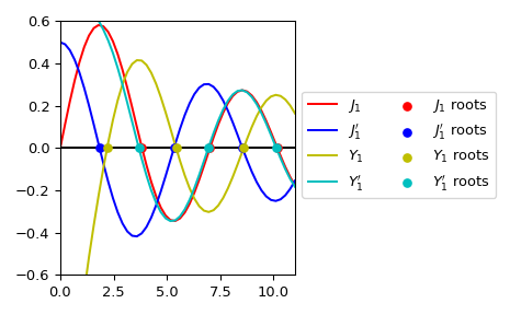
繪製 \(J_1\)、\(J_1'\)、\(Y_1\)、\(Y_1'\) 及其根。

>>> import numpy as np
>>> import matplotlib.pyplot as plt
>>> from scipy.special import jnyn_zeros, jvp, jn, yvp, yn
>>> jn_roots, jnp_roots, yn_roots, ynp_roots = jnyn_zeros(1, 3)
>>> fig, ax = plt.subplots()
>>> xmax= 11
>>> x = np.linspace(0, xmax)
>>> x[0] += 1e-15
>>> ax.plot(x, jn(1, x), label=r"$J_1$", c='r')
>>> ax.plot(x, jvp(1, x, 1), label=r"$J_1'$", c='b')
>>> ax.plot(x, yn(1, x), label=r"$Y_1$", c='y')
>>> ax.plot(x, yvp(1, x, 1), label=r"$Y_1'$", c='c')
>>> zeros = np.zeros((3, ))
>>> ax.scatter(jn_roots, zeros, s=30, c='r', zorder=5,
...            label=r"$J_1$ roots")
>>> ax.scatter(jnp_roots, zeros, s=30, c='b', zorder=5,
...            label=r"$J_1'$ roots")
>>> ax.scatter(yn_roots, zeros, s=30, c='y', zorder=5,
...            label=r"$Y_1$ roots")
>>> ax.scatter(ynp_roots, zeros, s=30, c='c', zorder=5,
...            label=r"$Y_1'$ roots")
>>> ax.hlines(0, 0, xmax, color='k')
>>> ax.set_ylim(-0.6, 0.6)
>>> ax.set_xlim(0, xmax)
>>> ax.legend(ncol=2, bbox_to_anchor=(1., 0.75))
>>> plt.tight_layout()
>>> plt.show()

返回在新分頁中開啟