root#
- scipy.optimize.root(fun, x0, args=(), method='hybr', jac=None, tol=None, callback=None, options=None)[source]#
尋找向量函數的根。
- 參數:
- funcallable
要尋找根的向量函數。
假設 callable 具有簽名
f0(x, *my_args, **my_kwargs),其中my_args和my_kwargs是必要的位置和關鍵字參數。與其傳遞f0作為 callable,不如將其包裝為僅接受x;例如,傳遞fun=lambda x: f0(x, *my_args, **my_kwargs)作為 callable,其中my_args(tuple) 和my_kwargs(dict) 已在此函數調用之前收集。- x0ndarray
初始猜測值。
- argstuple, optional
傳遞給目標函數及其 Jacobian 的額外參數。
- methodstr, optional
求解器類型。應為下列其中之一
- jacbool 或 callable, optional
如果 jac 是布林值且為 True,則假設 fun 除了目標函數外還會傳回 Jacobian 的值。如果為 False,則將以數值方式估計 Jacobian。jac 也可以是傳回 fun 的 Jacobian 的 callable。在這種情況下,它必須接受與 fun 相同的參數。
- tolfloat, optional
終止容忍度。若要進行詳細控制,請使用求解器特定的選項。
- callbackfunction, optional
選用的回呼函數。它在每次迭代時都會以
callback(x, f)的形式調用,其中 x 是目前的解,而 f 是對應的殘差。適用於 ‘hybr’ 和 ‘lm’ 以外的所有方法。- optionsdict, optional
求解器選項的字典。例如,xtol 或 maxiter,請參閱
show_options()以取得詳細資訊。
- 返回:
- solOptimizeResult
以
OptimizeResult物件表示的解。重要的屬性包括:x解陣列、success布林旗標,指示演算法是否成功退出,以及message描述終止原因。請參閱OptimizeResult以取得其他屬性的說明。
另請參閱
show_options求解器接受的其他選項
筆記
本節說明可透過 ‘method’ 參數選擇的可用求解器。預設方法為 hybr。
方法 hybr 使用 MINPACK [1] 中實作的 Powell 混合方法的修改版本。
方法 lm 使用 MINPACK [1] 中實作的 Levenberg-Marquardt 演算法的修改版本,以最小平方意義求解非線性方程式系統。
方法 df-sane 是一種無導數譜方法。[3]
方法 broyden1、broyden2、anderson、linearmixing、diagbroyden、excitingmixing、krylov 是不精確的牛頓法,具有回溯或完整線搜索 [2]。每種方法都對應於特定的 Jacobian 近似。
方法 broyden1 使用 Broyden 的第一個 Jacobian 近似,它被稱為 Broyden 的好方法。
方法 broyden2 使用 Broyden 的第二個 Jacobian 近似,它被稱為 Broyden 的壞方法。
方法 anderson 使用(擴展的)Anderson 混合。
方法 Krylov 使用 Krylov 近似來逼近逆 Jacobian。它適用於大規模問題。
方法 diagbroyden 使用對角 Broyden Jacobian 近似。
方法 linearmixing 使用純量 Jacobian 近似。
方法 excitingmixing 使用調整後的對角 Jacobian 近似。
警告
為方法 diagbroyden、linearmixing 和 excitingmixing 實作的演算法可能適用於特定問題,但它們是否有效可能很大程度上取決於問題。
在 0.11.0 版本中新增。
參考文獻
[2]C. T. Kelley。1995 年。《線性與非線性方程式的迭代方法》。工業與應用數學學會。 <https://archive.siam.org/books/kelley/fr16/>
[3]La Cruz, J.M. Martinez, M. Raydan。數學計算 75, 1429 (2006)。
範例
以下函數定義了非線性方程式系統及其 Jacobian。
>>> import numpy as np
>>> def fun(x):
...     return [x[0]  + 0.5 * (x[0] - x[1])**3 - 1.0,
...             0.5 * (x[1] - x[0])**3 + x[1]]
>>> def jac(x):
...     return np.array([[1 + 1.5 * (x[0] - x[1])**2,
...                       -1.5 * (x[0] - x[1])**2],
...                      [-1.5 * (x[1] - x[0])**2,
...                       1 + 1.5 * (x[1] - x[0])**2]])
可以透過以下方式獲得解。
>>> from scipy import optimize
>>> sol = optimize.root(fun, [0, 0], jac=jac, method='hybr')
>>> sol.x
array([ 0.8411639,  0.1588361])
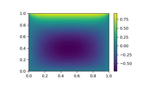
大型問題
假設我們需要在正方形 \([0,1]\times[0,1]\) 上求解以下積分微分方程式
\[\nabla^2 P = 10 \left(\int_0^1\int_0^1\cosh(P)\,dx\,dy\right)^2\]邊界條件為 \(P(x,1) = 1\),在正方形邊界的其他位置 \(P=0\)。
可以使用
method='krylov'求解器找到解>>> from scipy import optimize >>> # parameters >>> nx, ny = 75, 75 >>> hx, hy = 1./(nx-1), 1./(ny-1)
>>> P_left, P_right = 0, 0
>>> P_top, P_bottom = 1, 0
>>> def residual(P):
...    d2x = np.zeros_like(P)
...    d2y = np.zeros_like(P)
...
...    d2x[1:-1] = (P[2:]   - 2*P[1:-1] + P[:-2]) / hx/hx
...    d2x[0]    = (P[1]    - 2*P[0]    + P_left)/hx/hx
...    d2x[-1]   = (P_right - 2*P[-1]   + P[-2])/hx/hx
...
...    d2y[:,1:-1] = (P[:,2:] - 2*P[:,1:-1] + P[:,:-2])/hy/hy
...    d2y[:,0]    = (P[:,1]  - 2*P[:,0]    + P_bottom)/hy/hy
...    d2y[:,-1]   = (P_top   - 2*P[:,-1]   + P[:,-2])/hy/hy
...
...    return d2x + d2y - 10*np.cosh(P).mean()**2
>>> guess = np.zeros((nx, ny), float)
>>> sol = optimize.root(residual, guess, method='krylov')
>>> print('Residual: %g' % abs(residual(sol.x)).max())
Residual: 5.7972e-06  # may vary
>>> import matplotlib.pyplot as plt
>>> x, y = np.mgrid[0:1:(nx*1j), 0:1:(ny*1j)]
>>> plt.pcolormesh(x, y, sol.x, shading='gouraud')
>>> plt.colorbar()
>>> plt.show()