scipy.stats.studentized_range#
- scipy.stats.studentized_range = <scipy.stats._continuous_distns.studentized_range_gen object>[原始碼]#
學生化全距連續隨機變數。
作為
rv_continuous類別的實例,studentized_range物件繼承了它的一系列通用方法(完整列表請見下方),並以針對此特定分佈的詳細資訊來完善它們。另請參閱
t學生 t 分佈
筆記
對於
studentized_range的機率密度函數為\[f(x; k, \nu) = \frac{k(k-1)\nu^{\nu/2}}{\Gamma(\nu/2) 2^{\nu/2-1}} \int_{0}^{\infty} \int_{-\infty}^{\infty} s^{\nu} e^{-\nu s^2/2} \phi(z) \phi(sx + z) [\Phi(sx + z) - \Phi(z)]^{k-2} \,dz \,ds\]對於 \(x ≥ 0\)、\(k > 1\) 和 \(\nu > 0\)。
studentized_range接受k作為 \(k\) 和df作為 \(\nu\) 的形狀參數。當 \(\nu\) 超過 100,000 時,會使用漸近近似值(無限自由度)來計算累積分布函數 [4] 和機率分布函數。
上面的機率密度是以「標準化」形式定義的。若要平移和/或縮放分佈,請使用
loc和scale參數。具體而言,studentized_range.pdf(x, k, df, loc, scale)與studentized_range.pdf(y, k, df) / scale完全等效,其中y = (x - loc) / scale。請注意,平移分佈的位置不會使其成為「非中心」分佈;某些分佈的非中心化推廣在單獨的類別中提供。參考文獻
[2]Batista, Ben Dêivide, et al. “Externally Studentized Normal Midrange Distribution.” Ciência e Agrotecnologia, vol. 41, no. 4, 2017, pp. 378-389., doi:10.1590/1413-70542017414047716.
[3]Harter, H. Leon. “Tables of Range and Studentized Range.” The Annals of Mathematical Statistics, vol. 31, no. 4, 1960, pp. 1122-1147. JSTOR, www.jstor.org/stable/2237810. Accessed 18 Feb. 2021.
[4]Lund, R. E., and J. R. Lund. “Algorithm AS 190: Probabilities and Upper Quantiles for the Studentized Range.” Journal of the Royal Statistical Society. Series C (Applied Statistics), vol. 32, no. 2, 1983, pp. 204-210. JSTOR, www.jstor.org/stable/2347300. Accessed 18 Feb. 2021.
範例
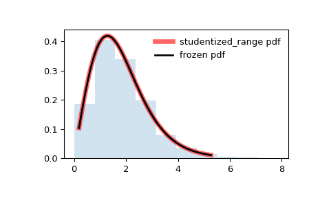
>>> import numpy as np
>>> from scipy.stats import studentized_range
>>> import matplotlib.pyplot as plt
>>> fig, ax = plt.subplots(1, 1)
顯示機率密度函數 (
pdf)>>> k, df = 3, 10 >>> x = np.linspace(studentized_range.ppf(0.01, k, df), ... studentized_range.ppf(0.99, k, df), 100) >>> ax.plot(x, studentized_range.pdf(x, k, df), ... 'r-', lw=5, alpha=0.6, label='studentized_range pdf')
或者,可以呼叫分佈物件(作為函數)來固定形狀、位置和比例參數。這會傳回一個「凍結」的 RV 物件,其中保存了給定的固定參數。
凍結分佈並顯示凍結的
pdf>>> rv = studentized_range(k, df) >>> ax.plot(x, rv.pdf(x), 'k-', lw=2, label='frozen pdf')
檢查
cdf和ppf的準確性>>> vals = studentized_range.ppf([0.001, 0.5, 0.999], k, df) >>> np.allclose([0.001, 0.5, 0.999], studentized_range.cdf(vals, k, df)) True
與其使用 (
studentized_range.rvs) 來產生隨機變數(對於此分佈而言速度非常慢),不如使用內插器來近似反向 CDF,然後使用此近似反向 CDF 執行反向轉換取樣。此分佈具有無限但細長的右尾,因此我們將注意力集中在最左邊的 99.9%。
>>> a, b = studentized_range.ppf([0, .999], k, df)
>>> a, b
0, 7.41058083802274
>>> from scipy.interpolate import interp1d
>>> rng = np.random.default_rng()
>>> xs = np.linspace(a, b, 50)
>>> cdf = studentized_range.cdf(xs, k, df)
# Create an interpolant of the inverse CDF
>>> ppf = interp1d(cdf, xs, fill_value='extrapolate')
# Perform inverse transform sampling using the interpolant
>>> r = ppf(rng.uniform(size=1000))
並比較直方圖
>>> ax.hist(r, density=True, histtype='stepfilled', alpha=0.2)
>>> ax.legend(loc='best', frameon=False)
>>> plt.show()
方法
rvs(k, df, loc=0, scale=1, size=1, random_state=None)
隨機變數。
pdf(x, k, df, loc=0, scale=1)
機率密度函數。
logpdf(x, k, df, loc=0, scale=1)
機率密度函數的對數。
cdf(x, k, df, loc=0, scale=1)
累積分布函數。
logcdf(x, k, df, loc=0, scale=1)
累積分布函數的對數。
sf(x, k, df, loc=0, scale=1)
存活函數(也定義為
1 - cdf,但 sf 有時更準確)。logsf(x, k, df, loc=0, scale=1)
存活函數的對數。
ppf(q, k, df, loc=0, scale=1)
百分點函數(
cdf的反函數 — 百分位數)。isf(q, k, df, loc=0, scale=1)
反向存活函數(
sf的反函數)。moment(order, k, df, loc=0, scale=1)
指定階數的非中心動差。
stats(k, df, loc=0, scale=1, moments=’mv’)
平均值 (‘m’)、變異數 (‘v’)、偏度 (‘s’) 和/或峰度 (‘k’)。
entropy(k, df, loc=0, scale=1)
RV 的(微分)熵。
fit(data)
通用資料的參數估計。請參閱 scipy.stats.rv_continuous.fit 以取得關鍵字引數的詳細文件。
expect(func, args=(k, df), loc=0, scale=1, lb=None, ub=None, conditional=False, **kwds)
函數(一個引數)關於分佈的期望值。
median(k, df, loc=0, scale=1)
分佈的中位數。
mean(k, df, loc=0, scale=1)
分佈的平均值。
var(k, df, loc=0, scale=1)
分佈的變異數。
std(k, df, loc=0, scale=1)
分佈的標準差。
interval(confidence, k, df, loc=0, scale=1)
具有圍繞中位數的相等面積的信賴區間。