scipy.stats.

sobol_indices#

scipy.stats.sobol_indices(*, func, n, dists=None, method='saltelli_2010', rng=None)[source]#

Sobol’ 全域敏感度指標。

參數:

func可呼叫物件或 dict(str, array_like)

如果 func 是可呼叫物件，則為用於計算 Sobol’ 指標的函數。其簽名必須為

func(x: ArrayLike) -> ArrayLike

其中 x 的形狀為 (d, n)，輸出形狀為 (s, n)，其中

d 是 func 的輸入維度（輸入變數的數量），
s 是 func 的輸出維度（輸出變數的數量），以及
n 是樣本數（請參閱下方的 n）。

函數評估值必須為有限值。

如果 func 是字典，則包含來自三個不同陣列的函數評估值。鍵必須為：f_A、f_B 和 f_AB。f_A 和 f_B 應具有形狀 (s, n)，而 f_AB 應具有形狀 (d, s, n)。這是一項進階功能，誤用可能會導致錯誤的分析。

nint

用於產生矩陣 A 和 B 的樣本數。必須為 2 的次方。將評估 func 的總點數將為 n*(d+2)。

distslist(distributions), optional

每個參數分佈的列表。參數的分佈取決於應用程式，應謹慎選擇。參數假設為獨立分佈，表示其值之間沒有約束或關係。

分佈必須為具有 ppf 方法的類別的實例。

如果 func 是可呼叫物件，則必須指定，否則將忽略。

methodCallable 或 str，預設值：‘saltelli_2010’

用於計算第一階和總階 Sobol’ 指標的方法。

如果為可呼叫物件，其簽名必須為

func(f_A: np.ndarray, f_B: np.ndarray, f_AB: np.ndarray)
-> Tuple[np.ndarray, np.ndarray]

其中 f_A, f_B 的形狀為 (s, n)，f_AB 的形狀為 (d, s, n)。這些陣列包含來自三組不同樣本的函數評估值。輸出是第一階和總階指標的元組，形狀為 (s, d)。這是一項進階功能，誤用可能會導致錯誤的分析。

rngnumpy.random.Generator, optional

虛擬隨機數產生器狀態。當 rng 為 None 時，將使用來自作業系統的熵建立新的 numpy.random.Generator。除了 numpy.random.Generator 之外的類型會傳遞至 numpy.random.default_rng 以實例化 Generator。

在版本 1.15.0 中變更：作為從使用 numpy.random.RandomState 過渡到 numpy.random.Generator 的 SPEC-007 過渡的一部分，此關鍵字已從 random_state 變更為 rng。在過渡期間，這兩個關鍵字將繼續運作，但一次只能指定一個。在過渡期之後，使用 random_state 關鍵字的函數呼叫將發出警告。在棄用期之後，將移除 random_state 關鍵字。

傳回值:

resSobolResult

具有屬性的物件

first_order形狀為 (s, d) 的 ndarray: 第一階 Sobol’ 指標。
total_order形狀為 (s, d) 的 ndarray: 總階 Sobol’ 指標。

以及方法

bootstrap(confidence_level: float, n_resamples: int) -> BootstrapSobolResult

一種提供指標信賴區間的方法。有關更多詳細資訊，請參閱 scipy.stats.bootstrap。

bootstrapping 是在第一階和總階指標上完成的，它們在 BootstrapSobolResult 中作為屬性 first_order 和 total_order 提供。

註解

Sobol’ 方法 [1]、[2] 是一種基於變異數的敏感度分析，可獲得每個參數對感興趣量 (QoI；即 func 的輸出) 的變異數的貢獻。各個貢獻可用於對參數進行排名，並透過計算模型的有效（或平均）維度來衡量模型的複雜性。

註解

參數假設為獨立分佈。每個參數仍然可以遵循任何分佈。實際上，分佈非常重要，應與參數的實際分佈相符。

它使用函數變異數的函數分解來探索

\[\mathbb{V}(Y) = \sum_{i}^{d} \mathbb{V}_i (Y) + \sum_{i<j}^{d} \mathbb{V}_{ij}(Y) + ... + \mathbb{V}_{1,2,...,d}(Y),\]

引入條件變異數

\[\mathbb{V}_i(Y) = \mathbb{\mathbb{V}}[\mathbb{E}(Y|x_i)] \qquad \mathbb{V}_{ij}(Y) = \mathbb{\mathbb{V}}[\mathbb{E}(Y|x_i x_j)] - \mathbb{V}_i(Y) - \mathbb{V}_j(Y),\]

Sobol’ 指標表示為

\[S_i = \frac{\mathbb{V}_i(Y)}{\mathbb{V}[Y]} \qquad S_{ij} =\frac{\mathbb{V}_{ij}(Y)}{\mathbb{V}[Y]}.\]

\(S_{i}\) 對應於一階項，該項評估第 i 個參數的貢獻，而 \(S_{ij}\) 對應於二階項，該項告知第 i 個和第 j 個參數之間互動的貢獻。這些方程式可以推廣以計算更高階項；但是，它們的計算成本很高，並且其解釋很複雜。這就是為什麼僅提供一階指標的原因。

總階指標表示參數對 QoI 變異數的全域貢獻，並定義為

\[S_{T_i} = S_i + \sum_j S_{ij} + \sum_{j,k} S_{ijk} + ... = 1 - \frac{\mathbb{V}[\mathbb{E}(Y|x_{\sim i})]}{\mathbb{V}[Y]}.\]

一階指標的總和小於或等於 1，而總階指標的總和至少為 1。如果沒有互動，則一階和總階指標相等，並且一階和總階指標的總和均為 1。

警告

負 Sobol’ 值是由於數值錯誤造成的。增加點數 n 應有助於解決此問題。

進行良好分析所需的樣本數會隨著問題的維度而增加。例如，對於 3 維問題，請考慮至少 n >= 2**12。模型越複雜，需要的樣本就越多。

即使對於純粹的加法模型，由於數值雜訊，指標的總和也可能不為 1。

參考文獻

[1]

Sobol, I. M.。 “非線性數學模型的敏感度分析。” Mathematical Modeling and Computational Experiment, 1:407-414, 1993。

[2]

Sobol, I. M. (2001)。 “非線性數學模型及其蒙地卡羅估計的全域敏感度指標。” Mathematics and Computers in Simulation, 55(1-3):271-280, DOI:10.1016/S0378-4754(00)00270-6, 2001。

[3]

Saltelli, A.。 “充分利用模型評估來計算敏感度指標。” Computer Physics Communications, 145(2):280-297, DOI:10.1016/S0010-4655(02)00280-1, 2002。

[4]

Saltelli, A.、M. Ratto、T. Andres、F. Campolongo、J. Cariboni、D. Gatelli、M. Saisana 和 S. Tarantola。“全域敏感度分析。《入門指南》。” 2007。

[5]

Saltelli, A.、P. Annoni、I. Azzini、F. Campolongo、M. Ratto 和 S. Tarantola。“模型輸出的基於變異數的敏感度分析。總敏感度指標的設計和估計器。” Computer Physics Communications, 181(2):259-270, DOI:10.1016/j.cpc.2009.09.018, 2010。

[6]

Ishigami, T. 和 T. Homma。“電腦模型不確定性分析中的重要性量化技術。” IEEE, DOI:10.1109/ISUMA.1990.151285, 1990。

範例

以下是 Ishigami 函數的範例 [6]

\[Y(\mathbf{x}) = \sin x_1 + 7 \sin^2 x_2 + 0.1 x_3^4 \sin x_1,\]

其中 \(\mathbf{x} \in [-\pi, \pi]^3\)。此函數表現出強烈的非線性和非單調性。

請記住，Sobol’ 指標假設樣本是獨立分佈的。在本例中，我們在每個邊際上使用均勻分佈。

>>> import numpy as np
>>> from scipy.stats import sobol_indices, uniform
>>> rng = np.random.default_rng()
>>> def f_ishigami(x):
...     f_eval = (
...         np.sin(x[0])
...         + 7 * np.sin(x[1])**2
...         + 0.1 * (x[2]**4) * np.sin(x[0])
...     )
...     return f_eval
>>> indices = sobol_indices(
...     func=f_ishigami, n=1024,
...     dists=[
...         uniform(loc=-np.pi, scale=2*np.pi),
...         uniform(loc=-np.pi, scale=2*np.pi),
...         uniform(loc=-np.pi, scale=2*np.pi)
...     ],
...     rng=rng
... )
>>> indices.first_order
array([0.31637954, 0.43781162, 0.00318825])
>>> indices.total_order
array([0.56122127, 0.44287857, 0.24229595])

可以使用 bootstrapping 獲得信賴區間。

>>> boot = indices.bootstrap()

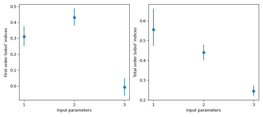
然後，可以輕鬆地將此資訊視覺化。

>>> import matplotlib.pyplot as plt
>>> fig, axs = plt.subplots(1, 2, figsize=(9, 4))
>>> _ = axs[0].errorbar(
...     [1, 2, 3], indices.first_order, fmt='o',
...     yerr=[
...         indices.first_order - boot.first_order.confidence_interval.low,
...         boot.first_order.confidence_interval.high - indices.first_order
...     ],
... )
>>> axs[0].set_ylabel("First order Sobol' indices")
>>> axs[0].set_xlabel('Input parameters')
>>> axs[0].set_xticks([1, 2, 3])
>>> _ = axs[1].errorbar(
...     [1, 2, 3], indices.total_order, fmt='o',
...     yerr=[
...         indices.total_order - boot.total_order.confidence_interval.low,
...         boot.total_order.confidence_interval.high - indices.total_order
...     ],
... )
>>> axs[1].set_ylabel("Total order Sobol' indices")
>>> axs[1].set_xlabel('Input parameters')
>>> axs[1].set_xticks([1, 2, 3])
>>> plt.tight_layout()
>>> plt.show()

../../_images/scipy-stats-sobol_indices-1_00_00.png

註解

預設情況下，scipy.stats.uniform 的支援為 [0, 1]。使用參數 loc 和 scale，可以獲得 [loc, loc + scale] 上的均勻分佈。

此結果特別有趣，因為一階指標 \(S_{x_3} = 0\)，而其總階指標為 \(S_{T_{x_3}} = 0.244\)。這表示與 \(x_3\) 的更高階互動是造成差異的原因。\(x_3\) 與 \(x_1\) 之間的相關性導致 QoI 上觀察到的變異數幾乎有 25%，儘管 \(x_3\) 本身對 QoI 沒有影響。

以下是此函數上 Sobol’ 指標的視覺解釋。讓我們在 \([-\pi, \pi]^3\) 中產生 1024 個樣本，並計算輸出值。

>>> from scipy.stats import qmc
>>> n_dim = 3
>>> p_labels = ['$x_1$', '$x_2$', '$x_3$']
>>> sample = qmc.Sobol(d=n_dim, seed=rng).random(1024)
>>> sample = qmc.scale(
...     sample=sample,
...     l_bounds=[-np.pi, -np.pi, -np.pi],
...     u_bounds=[np.pi, np.pi, np.pi]
... )
>>> output = f_ishigami(sample.T)

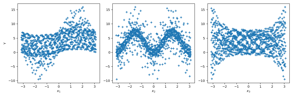
現在我們可以繪製輸出相對於每個參數的散佈圖。這提供了一種視覺方式來理解每個參數如何影響函數的輸出。

>>> fig, ax = plt.subplots(1, n_dim, figsize=(12, 4))
>>> for i in range(n_dim):
...     xi = sample[:, i]
...     ax[i].scatter(xi, output, marker='+')
...     ax[i].set_xlabel(p_labels[i])
>>> ax[0].set_ylabel('Y')
>>> plt.tight_layout()
>>> plt.show()

../../_images/scipy-stats-sobol_indices-1_01_00.png

現在 Sobol’ 更進一步：透過將輸出值以給定參數值（黑線）為條件，計算條件輸出平均值。它對應於項 \(\mathbb{E}(Y|x_i)\)。取此項的變異數會得到 Sobol’ 指標的分子。

>>> mini = np.min(output)
>>> maxi = np.max(output)
>>> n_bins = 10
>>> bins = np.linspace(-np.pi, np.pi, num=n_bins, endpoint=False)
>>> dx = bins[1] - bins[0]
>>> fig, ax = plt.subplots(1, n_dim, figsize=(12, 4))
>>> for i in range(n_dim):
...     xi = sample[:, i]
...     ax[i].scatter(xi, output, marker='+')
...     ax[i].set_xlabel(p_labels[i])
...     for bin_ in bins:
...         idx = np.where((bin_ <= xi) & (xi <= bin_ + dx))
...         xi_ = xi[idx]
...         y_ = output[idx]
...         ave_y_ = np.mean(y_)
...         ax[i].plot([bin_ + dx/2] * 2, [mini, maxi], c='k')
...         ax[i].scatter(bin_ + dx/2, ave_y_, c='r')
>>> ax[0].set_ylabel('Y')
>>> plt.tight_layout()
>>> plt.show()

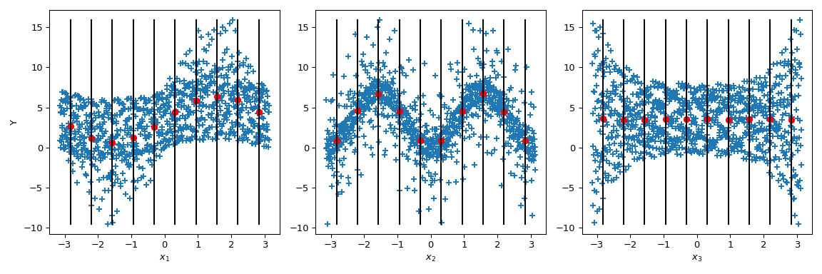
../../_images/scipy-stats-sobol_indices-1_02_00.png

查看 \(x_3\)，平均值的變異數為零，導致 \(S_{x_3} = 0\)。但是我們可以進一步觀察到，輸出值的變異數沿著 \(x_3\) 的參數值不是恆定的。這種異質變異數性是由更高階互動解釋的。此外，在 \(x_1\) 上也可以注意到異質變異數性，導致 \(x_3\) 和 \(x_1\) 之間發生互動。在 \(x_2\) 上，變異數似乎是恆定的，因此可以假設與此參數的互動為零。

這種情況很容易進行視覺分析，儘管這只是一種定性分析。儘管如此，當輸入參數的數量增加時，這種分析變得不切實際，因為很難對高階項得出結論。因此，使用 Sobol’ 指標的好處就顯現出來了。