scipy.stats.

ppcc_max#

scipy.stats.ppcc_max(x, brack=(0.0, 1.0), dist='tukeylambda')[原始碼]#

計算最大化 PPCC 的形狀參數。

機率圖相關係數 (PPCC) 圖可用於確定單參數分佈族的最優形狀參數。ppcc_max 返回將最大化給定數據到單參數分佈族的機率圖相關係數的形狀參數。

參數:

xarray_like: 輸入陣列。
bracktuple, optional: 三元組 (a,b,c)，其中 (a<b<c)。如果括號由兩個數字 (a, c) 組成，則它們被假定為下坡括號搜尋的起始區間 (請參閱 scipy.optimize.brent)。
diststr 或 stats.distributions 實例，選填: 分佈或分佈函數名稱。外觀與 stats.distributions 實例足夠相似的物件 (即它們具有 ppf 方法) 也被接受。預設值為 'tukeylambda'。

回傳值:

shape_valuefloat: 機率圖相關係數達到最大值的形狀參數。

參見

ppcc_plot、probplot、boxcox

註解

brack 關鍵字作為起點，在邊角情況下很有用。可以使用圖表來獲得最大值位置的粗略視覺估計，以便在其附近開始搜尋。

參考文獻

[1]

J.J. Filliben, “常態性機率圖相關係數檢定”, Technometrics, Vol. 17, pp. 111-117, 1975.

[2]

工程統計手冊, NIST/SEMATEC, https://www.itl.nist.gov/div898/handbook/eda/section3/ppccplot.htm

範例

首先，我們從形狀參數為 2.5 的 Weibull 分佈中產生一些隨機數據

>>> import numpy as np
>>> from scipy import stats
>>> import matplotlib.pyplot as plt
>>> rng = np.random.default_rng()
>>> c = 2.5
>>> x = stats.weibull_min.rvs(c, scale=4, size=2000, random_state=rng)

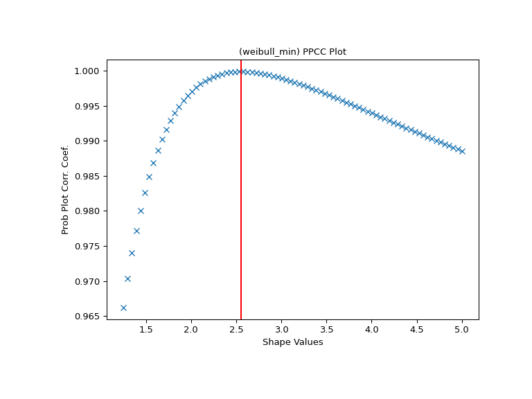
使用 Weibull 分佈為此數據產生 PPCC 圖。

>>> fig, ax = plt.subplots(figsize=(8, 6))
>>> res = stats.ppcc_plot(x, c/2, 2*c, dist='weibull_min', plot=ax)

我們計算形狀應達到最大值的值，並在那裡繪製一條紅線。該線應與 PPCC 圖中的最高點重合。

>>> cmax = stats.ppcc_max(x, brack=(c/2, 2*c), dist='weibull_min')
>>> ax.axvline(cmax, color='r')
>>> plt.show()

../../_images/scipy-stats-ppcc_max-1.png