scipy.stats.

ppcc_plot

scipy.stats.ppcc_plot(x, a, b, dist='tukeylambda', plot=None, N=80)

計算並可選繪製機率圖相關係數。

機率圖相關係數 (PPCC) 圖可用於確定單參數分佈族的最優形狀參數。它不能用於沒有形狀參數（如常態分佈）或具有多個形狀參數的分佈。

預設情況下，使用 Tukey-Lambda 分佈 (stats.tukeylambda)。Tukey-Lambda PPCC 圖通過近似常態分佈從長尾分佈插值到短尾分佈，因此在實務中特別有用。

參數:

xarray_like

輸入陣列。

a, bscalar

要使用的形狀參數的下限和上限。

diststr 或 stats.distributions 實例, 可選

分佈或分佈函數名稱。看起來很像 stats.distributions 實例的物件（即它們具有 ppf 方法）也被接受。預設值為 'tukeylambda'。

plot物件, 可選

如果給定，則繪製 PPCC 對形狀參數的圖。plot 是一個必須具有 “plot” 和 “text” 方法的物件。可以使用 matplotlib.pyplot 模組或 Matplotlib Axes 物件，或具有相同方法的自訂物件。預設值為 None，這表示不建立任何圖表。

Nint, 可選

水平軸上的點數（從 a 到 b 均勻分佈）。

返回:

svalsndarray

計算 ppcc 的形狀值。

ppccndarray

計算的機率圖相關係數值。

參見

ppcc_max, probplot, boxcox_normplot, tukeylambda

參考文獻

J.J. Filliben, “常態性的機率圖相關係數檢定”, Technometrics, Vol. 17, pp. 111-117, 1975.

範例

在您的瀏覽器中試試看！

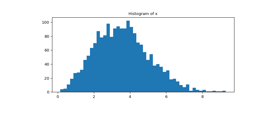
首先，我們從形狀參數為 2.5 的 Weibull 分佈生成一些隨機資料，並繪製資料的直方圖

>>> import numpy as np
>>> from scipy import stats
>>> import matplotlib.pyplot as plt
>>> rng = np.random.default_rng()
>>> c = 2.5
>>> x = stats.weibull_min.rvs(c, scale=4, size=2000, random_state=rng)

看看資料的直方圖。

>>> fig1, ax = plt.subplots(figsize=(9, 4))
>>> ax.hist(x, bins=50)
>>> ax.set_title('Histogram of x')
>>> plt.show()

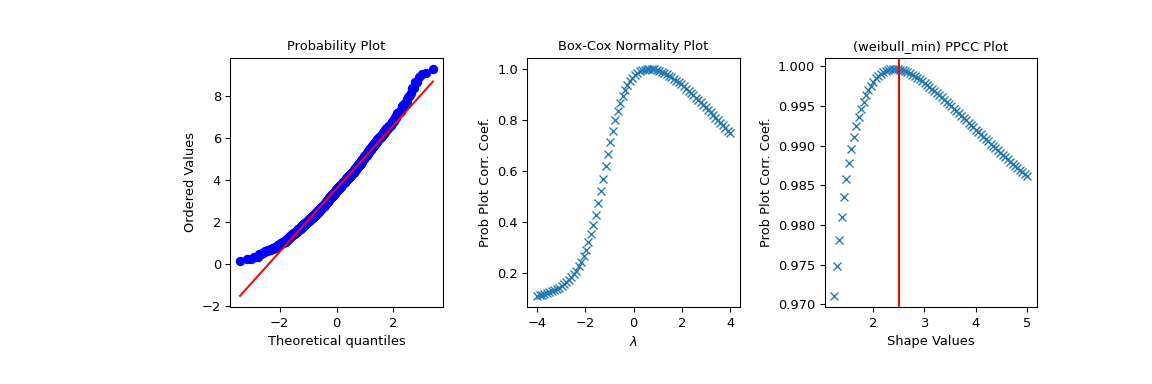
現在，我們使用 PPCC 圖以及相關的機率圖和 Box-Cox 常態圖來探索這些資料。繪製一條紅線，標示我們預期 PPCC 值達到最大值的位置（在上面使用的形狀參數 c 處）

>>> fig2 = plt.figure(figsize=(12, 4))
>>> ax1 = fig2.add_subplot(1, 3, 1)
>>> ax2 = fig2.add_subplot(1, 3, 2)
>>> ax3 = fig2.add_subplot(1, 3, 3)
>>> res = stats.probplot(x, plot=ax1)
>>> res = stats.boxcox_normplot(x, -4, 4, plot=ax2)
>>> res = stats.ppcc_plot(x, c/2, 2*c, dist='weibull_min', plot=ax3)
>>> ax3.axvline(c, color='r')
>>> plt.show()

返回在新分頁中開啟