scipy.stats.irwinhall#
- scipy.stats.irwinhall = <scipy.stats._continuous_distns.irwinhall_gen object>[source]#
Irwin-Hall(均勻總和)連續隨機變數。
Irwin-Hall 連續隨機變數是 \(n\) 個獨立標準均勻隨機變數的總和 [1] [2]。
作為
rv_continuous類別的一個實例,irwinhall物件繼承了它的一系列通用方法(完整列表請見下方),並用針對此特定分佈的詳細資訊完善了它們。註解
應用包括 Rao 的間隔檢定,當資料不是單峰時,它是 Rayleigh 檢定更強大的替代方案,以及雷達 [3]。
方便的是,pdf 和 cdf 是標準均勻分佈的 \(n\) 折疊積,這也是基數 B 樣條的定義,其階數為 \(n-1\),節點均勻間隔從 \(1\) 到 \(n\) [4] [5]。
Bates 分佈,它表示統計獨立、均勻分佈的隨機變數的平均值,僅僅是 Irwin-Hall 分佈按 \(1/n\) 縮放的結果。例如,凍結分佈
bates = irwinhall(10, scale=1/10)表示 10 個均勻分佈的隨機變數的平均值分佈。上面的機率密度是以「標準化」形式定義的。若要平移和/或縮放分佈,請使用
loc和scale參數。具體來說,irwinhall.pdf(x, n, loc, scale)與irwinhall.pdf(y, n) / scale完全等效,其中y = (x - loc) / scale。請注意,平移分佈的位置不會使其成為「非中心」分佈;某些分佈的非中心推廣版本在單獨的類別中提供。參考文獻
[1]P. Hall, “The distribution of means for samples of size N drawn from a population in which the variate takes values between 0 and 1, all such values being equally probable”, Biometrika, Volume 19, Issue 3-4, December 1927, Pages 240-244, DOI:10.1093/biomet/19.3-4.240.
[2]J. O. Irwin, “On the frequency distribution of the means of samples from a population having any law of frequency with finite moments, with special reference to Pearson’s Type II, Biometrika, Volume 19, Issue 3-4, December 1927, Pages 225-239, DOI:0.1093/biomet/19.3-4.225.
[3]K. Buchanan, T. Adeyemi, C. Flores-Molina, S. Wheeland and D. Overturf, “Sidelobe behavior and bandwidth characteristics of distributed antenna arrays,” 2018 United States National Committee of URSI National Radio Science Meeting (USNC-URSI NRSM), Boulder, CO, USA, 2018, pp. 1-2. https://www.usnc-ursi-archive.org/nrsm/2018/papers/B15-9.pdf.
[4]Amos Ron, “Lecture 1: Cardinal B-splines and convolution operators”, p. 1 https://pages.cs.wisc.edu/~deboor/887/lec1new.pdf.
[5]Trefethen, N. (2012, July). B-splines and convolution. Chebfun. Retrieved April 30, 2024, from http://www.chebfun.org/examples/approx/BSplineConv.html.
範例
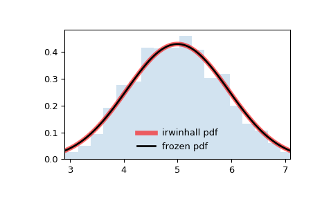
>>> import numpy as np
>>> from scipy.stats import irwinhall
>>> import matplotlib.pyplot as plt
>>> fig, ax = plt.subplots(1, 1)
計算前四個動差
>>> n = 10
>>> mean, var, skew, kurt = irwinhall.stats(n, moments='mvsk')
顯示機率密度函數 (
pdf)>>> x = np.linspace(irwinhall.ppf(0.01, n), ... irwinhall.ppf(0.99, n), 100) >>> ax.plot(x, irwinhall.pdf(x, n), ... 'r-', lw=5, alpha=0.6, label='irwinhall pdf')
或者,可以呼叫分佈物件(作為函數)以固定形狀、位置和縮放參數。這會傳回一個「凍結」的 RV 物件,其中包含給定的固定參數。
凍結分佈並顯示凍結的
pdf>>> rv = irwinhall(n) >>> ax.plot(x, rv.pdf(x), 'k-', lw=2, label='frozen pdf')
檢查
cdf和ppf的準確性>>> vals = irwinhall.ppf([0.001, 0.5, 0.999], n) >>> np.allclose([0.001, 0.5, 0.999], irwinhall.cdf(vals, n)) True
產生隨機數字
>>> r = irwinhall.rvs(n, size=1000)
並比較直方圖
>>> ax.hist(r, density=True, bins='auto', histtype='stepfilled', alpha=0.2)
>>> ax.set_xlim([x[0], x[-1]])
>>> ax.legend(loc='best', frameon=False)
>>> plt.show()
方法
rvs(n, loc=0, scale=1, size=1, random_state=None)
隨機變數。
pdf(x, n, loc=0, scale=1)
機率密度函數。
logpdf(x, n, loc=0, scale=1)
機率密度函數的對數。
cdf(x, n, loc=0, scale=1)
累積分布函數。
logcdf(x, n, loc=0, scale=1)
累積分布函數的對數。
sf(x, n, loc=0, scale=1)
存活函數(也定義為
1 - cdf,但 sf 有時更準確)。logsf(x, n, loc=0, scale=1)
存活函數的對數。
ppf(q, n, loc=0, scale=1)
百分點函數(
cdf的反函數 — 百分位數)。isf(q, n, loc=0, scale=1)
反向存活函數(
sf的反函數)。moment(order, n, loc=0, scale=1)
指定階數的非中心動差。
stats(n, loc=0, scale=1, moments=’mv’)
平均值 ('m')、變異數 ('v')、偏度 ('s') 和/或峰度 ('k')。
entropy(n, loc=0, scale=1)
RV 的(微分)熵。
fit(data)
通用資料的參數估計。 有關關鍵字引數的詳細文件,請參閱 scipy.stats.rv_continuous.fit。
expect(func, args=(n,), loc=0, scale=1, lb=None, ub=None, conditional=False, **kwds)
關於分佈的函數(一個引數)的期望值。
median(n, loc=0, scale=1)
分佈的中位數。
mean(n, loc=0, scale=1)
分佈的平均值。
var(n, loc=0, scale=1)
分佈的變異數。
std(n, loc=0, scale=1)
分佈的標準差。
interval(confidence, n, loc=0, scale=1)
中位數周圍區域相等的信賴區間。