scipy.special.

y1p_zeros

scipy.special.y1p_zeros(nt, complex=False)

計算 Bessel 導函數 Y1’(z) 的 nt 個零點，以及每個零點的值。

這些值由 Y1(z1) 在每個 Y1’(z1)=0 的 z1 給出。

參數:

ntint

要返回的零點數量

complexbool, 預設為 False

設定為 False 以僅返回實數零點；設定為 True 以僅返回具有負實部和正虛部的複數零點。 請注意，後者的複共軛也是函數的零點，但此常式不會返回。

返回:

z1pnndarray

Y1’(z) 第 n 個零點的位置

y1z1pnndarray

第 n 個零點的導函數 Y1(z1) 值

參考文獻

[1]

Zhang, Shanjie and Jin, Jianming. “Computation of Special Functions”, John Wiley and Sons, 1996, chapter 5. https://people.sc.fsu.edu/~jburkardt/f77_src/special_functions/special_functions.html

範例

在您的瀏覽器中試試看！

計算 \(Y_1'\) 的前四個根，以及 \(Y_1\) 在這些根上的值。

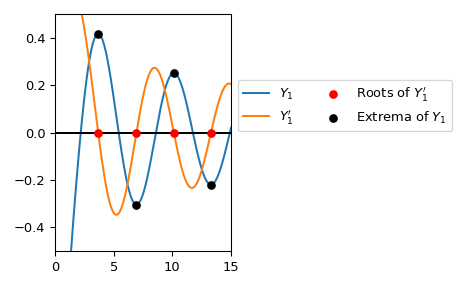
>>> import numpy as np
>>> from scipy.special import y1p_zeros
>>> y1grad_roots, y1_values = y1p_zeros(4)
>>> with np.printoptions(precision=5):
...     print(f"Y1' Roots: {y1grad_roots.real}")
...     print(f"Y1 values: {y1_values.real}")
Y1' Roots: [ 3.68302  6.9415  10.1234  13.28576]
Y1 values: [ 0.41673 -0.30317  0.25091 -0.21897]

y1p_zeros 可用於直接計算 \(Y_1\) 的極值點。 在此我們繪製 \(Y_1\) 和前四個極值。

>>> import matplotlib.pyplot as plt
>>> from scipy.special import y1, yvp
>>> y1_roots, y1_values_at_roots = y1p_zeros(4)
>>> real_roots = y1_roots.real
>>> xmax = 15
>>> x = np.linspace(0, xmax, 500)
>>> x[0] += 1e-15
>>> fig, ax = plt.subplots()
>>> ax.plot(x, y1(x), label=r'$Y_1$')
>>> ax.plot(x, yvp(1, x, 1), label=r"$Y_1'$")
>>> ax.scatter(real_roots, np.zeros((4, )), s=30, c='r',
...            label=r"Roots of $Y_1'$", zorder=5)
>>> ax.scatter(real_roots, y1_values_at_roots.real, s=30, c='k',
...            label=r"Extrema of $Y_1$", zorder=5)
>>> ax.hlines(0, 0, xmax, color='k')
>>> ax.set_ylim(-0.5, 0.5)
>>> ax.set_xlim(0, xmax)
>>> ax.legend(ncol=2, bbox_to_anchor=(1., 0.75))
>>> plt.tight_layout()
>>> plt.show()

返回在新分頁中開啟