scipy.special.

y1_zeros

scipy.special.y1_zeros(nt, complex=False)

計算 Bessel 函數 Y1(z) 的 nt 個零點，以及每個零點的導數。

導數由 Y1’(z1) = Y0(z1) 在每個零點 z1 給出。

參數:

ntint

要返回的零點數量

complexbool，預設為 False

設定為 False 僅返回實數零點；設定為 True 僅返回實部為負且虛部為正的複數零點。請注意，後者的共軛複數也是函數的零點，但此常式不會返回。

返回:

z1nndarray

Y1(z) 的第 n 個零點的位置

y1pz1nndarray

第 n 個零點的導數 Y1’(z1) 的值

參考文獻

[1]

Zhang, Shanjie and Jin, Jianming. “Computation of Special Functions”, John Wiley and Sons, 1996, chapter 5. https://people.sc.fsu.edu/~jburkardt/f77_src/special_functions/special_functions.html

範例

在瀏覽器中試試看！

計算 \(Y_1\) 的前 4 個實根以及根的導數

>>> import numpy as np
>>> from scipy.special import y1_zeros
>>> zeros, grads = y1_zeros(4)
>>> with np.printoptions(precision=5):
...     print(f"Roots: {zeros}")
...     print(f"Gradients: {grads}")
Roots: [ 2.19714+0.j  5.42968+0.j  8.59601+0.j 11.74915+0.j]
Gradients: [ 0.52079+0.j -0.34032+0.j  0.27146+0.j -0.23246+0.j]

提取實部

>>> realzeros = zeros.real
>>> realzeros
array([ 2.19714133,  5.42968104,  8.59600587, 11.74915483])

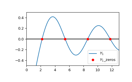
繪製 \(Y_1\) 和前四個計算出的根。

>>> import matplotlib.pyplot as plt
>>> from scipy.special import y1
>>> xmin = 0
>>> xmax = 13
>>> x = np.linspace(xmin, xmax, 500)
>>> zeros, grads = y1_zeros(4)
>>> fig, ax = plt.subplots()
>>> ax.hlines(0, xmin, xmax, color='k')
>>> ax.plot(x, y1(x), label=r'$Y_1$')
>>> ax.scatter(zeros.real, np.zeros((4, )), s=30, c='r',
...            label=r'$Y_1$_zeros', zorder=5)
>>> ax.set_ylim(-0.5, 0.5)
>>> ax.set_xlim(xmin, xmax)
>>> plt.legend()
>>> plt.show()

透過設定 complex=True 來計算 \(Y_1\) 的前 4 個複數根以及根的導數

>>> y1_zeros(4, True)
(array([ -0.50274327+0.78624371j,  -3.83353519+0.56235654j,
         -7.01590368+0.55339305j, -10.17357383+0.55127339j]),
 array([-0.45952768+1.31710194j,  0.04830191-0.69251288j,
        -0.02012695+0.51864253j,  0.011614  -0.43203296j]))

返回在新分頁中開啟