scipy.special.

y0_zeros

scipy.special.y0_zeros(nt, complex=False)

計算貝索函數 Y0(z) 的 nt 個零點，以及每個零點的導數。

導數在每個零點 z0 由 Y0’(z0) = -Y1(z0) 給出。

參數:

ntint

要返回的零點數量

complexbool, 預設值 False

設定為 False 以僅返回實數零點；設定為 True 以僅返回具有負實部和正虛部的複數零點。請注意，後者的複數共軛也是函數的零點，但此常式不會返回它們。

返回:

z0nndarray

Y0(z) 的第 n 個零點的位置

y0pz0nndarray

第 n 個零點的導數 Y0’(z0) 的值

參考文獻

[1]

Zhang, Shanjie and Jin, Jianming. “Computation of Special Functions”, John Wiley and Sons, 1996, chapter 5. https://people.sc.fsu.edu/~jburkardt/f77_src/special_functions/special_functions.html

範例

在您的瀏覽器中試試看！

計算 \(Y_0\) 的前 4 個實根以及根的導數

>>> import numpy as np
>>> from scipy.special import y0_zeros
>>> zeros, grads = y0_zeros(4)
>>> with np.printoptions(precision=5):
...     print(f"Roots: {zeros}")
...     print(f"Gradients: {grads}")
Roots: [ 0.89358+0.j  3.95768+0.j  7.08605+0.j 10.22235+0.j]
Gradients: [-0.87942+0.j  0.40254+0.j -0.3001 +0.j  0.2497 +0.j]

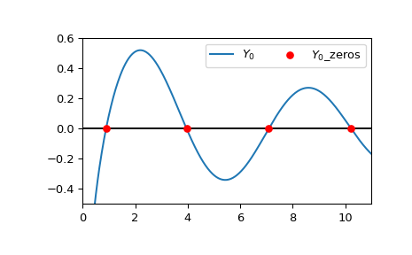
繪製 \(Y_0\) 的實部和前四個計算出的根。

>>> import matplotlib.pyplot as plt
>>> from scipy.special import y0
>>> xmin = 0
>>> xmax = 11
>>> x = np.linspace(xmin, xmax, 500)
>>> fig, ax = plt.subplots()
>>> ax.hlines(0, xmin, xmax, color='k')
>>> ax.plot(x, y0(x), label=r'$Y_0$')
>>> zeros, grads = y0_zeros(4)
>>> ax.scatter(zeros.real, np.zeros((4, )), s=30, c='r',
...            label=r'$Y_0$_zeros', zorder=5)
>>> ax.set_ylim(-0.5, 0.6)
>>> ax.set_xlim(xmin, xmax)
>>> plt.legend(ncol=2)
>>> plt.show()

透過設定 complex=True 來計算 \(Y_0\) 的前 4 個複數根以及根的導數

>>> y0_zeros(4, True)
(array([ -2.40301663+0.53988231j,  -5.5198767 +0.54718001j,
         -8.6536724 +0.54841207j, -11.79151203+0.54881912j]),
 array([ 0.10074769-0.88196771j, -0.02924642+0.5871695j ,
         0.01490806-0.46945875j, -0.00937368+0.40230454j]))

返回在新分頁中開啟