scipy.special.
spherical_jn#
- scipy.special.spherical_jn(n, z, derivative=False)[source]#
第一類球貝索函數或其導數。
定義為 [1],
\[j_n(z) = \sqrt{\frac{\pi}{2z}} J_{n + 1/2}(z),\]其中 \(J_n\) 是第一類貝索函數。
- 參數:
- nint, 類陣列
貝索函數的階數 (n >= 0)。
- z複數或浮點數,類陣列
貝索函數的自變數。
- derivativebool,選用
如果為 True,則返回導數的值(而非函數本身)。
- 返回:
- jnndarray
註解
對於大於階數的實數自變數,此函數使用升冪遞迴關係式 [2] 計算。對於小的實數或複數自變數,則使用與第一類柱貝索函數的定義關係。
導數是使用關係式 [3] 計算,
\[ \begin{align}\begin{aligned}j_n'(z) = j_{n-1}(z) - \frac{n + 1}{z} j_n(z).\\j_0'(z) = -j_1(z)\end{aligned}\end{align} \]Added in version 0.18.0.
參考文獻
[AS]Milton Abramowitz and Irene A. Stegun, eds. Handbook of Mathematical Functions with Formulas, Graphs, and Mathematical Tables. New York: Dover, 1972.
範例
第一類球貝索函數 \(j_n\) 接受實數和複數第二個自變數。它們可以返回複數類型
>>> from scipy.special import spherical_jn
>>> spherical_jn(0, 3+5j)
(-9.878987731663194-8.021894345786002j)
>>> type(spherical_jn(0, 3+5j))
<class 'numpy.complex128'>
我們可以從 \(n=3\) 在區間 \([1, 2]\) 的註解中驗證導數的關係式
>>> import numpy as np
>>> x = np.arange(1.0, 2.0, 0.01)
>>> np.allclose(spherical_jn(3, x, True),
...             spherical_jn(2, x) - 4/x * spherical_jn(3, x))
True
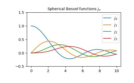
前幾個帶有實數自變數的 \(j_n\)
>>> import matplotlib.pyplot as plt
>>> x = np.arange(0.0, 10.0, 0.01)
>>> fig, ax = plt.subplots()
>>> ax.set_ylim(-0.5, 1.5)
>>> ax.set_title(r'Spherical Bessel functions $j_n$')
>>> for n in np.arange(0, 4):
...     ax.plot(x, spherical_jn(n, x), label=rf'$j_{n}$')
>>> plt.legend(loc='best')
>>> plt.show()