scipy.special.itairy#
- scipy.special.itairy(x, out=None) = <ufunc 'itairy'>#
Airy 函數的積分
計算從 0 到 x 的 Airy 函數積分。
- 參數:
- xarray_like
積分上限 (float)。
- outtuple of ndarray, optional
函數值的可選輸出陣列
- 返回:
- Aptscalar or ndarray
Ai(t) 從 0 到 x 的積分。
- Bptscalar or ndarray
Bi(t) 從 0 到 x 的積分。
- Antscalar or ndarray
Ai(-t) 從 0 到 x 的積分。
- Bntscalar or ndarray
Bi(-t) 從 0 到 x 的積分。
註解
由 Shanjie Zhang 和 Jianming Jin 創建的 Fortran 常式包裝器 [1]。
參考文獻
[1]Zhang, Shanjie and Jin, Jianming. “Computation of Special Functions”, John Wiley and Sons, 1996. https://people.sc.fsu.edu/~jburkardt/f_src/special_functions/special_functions.html
範例
計算
x=1.的函數值。>>> import numpy as np >>> from scipy.special import itairy >>> import matplotlib.pyplot as plt >>> apt, bpt, ant, bnt = itairy(1.) >>> apt, bpt, ant, bnt (0.23631734191710949, 0.8727691167380077, 0.46567398346706845, 0.3730050096342943)
通過為 x 提供 NumPy 陣列來計算多個點的函數值。
>>> x = np.array([1., 1.5, 2.5, 5])
>>> apt, bpt, ant, bnt = itairy(x)
>>> apt, bpt, ant, bnt
(array([0.23631734, 0.28678675, 0.324638  , 0.33328759]),
 array([  0.87276912,   1.62470809,   5.20906691, 321.47831857]),
 array([0.46567398, 0.72232876, 0.93187776, 0.7178822 ]),
 array([ 0.37300501,  0.35038814, -0.02812939,  0.15873094]))
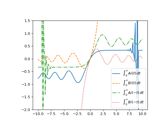
繪製從 -10 到 10 的函數圖。
>>> x = np.linspace(-10, 10, 500)
>>> apt, bpt, ant, bnt = itairy(x)
>>> fig, ax = plt.subplots(figsize=(6, 5))
>>> ax.plot(x, apt, label=r"$\int_0^x\, Ai(t)\, dt$")
>>> ax.plot(x, bpt, ls="dashed", label=r"$\int_0^x\, Bi(t)\, dt$")
>>> ax.plot(x, ant, ls="dashdot", label=r"$\int_0^x\, Ai(-t)\, dt$")
>>> ax.plot(x, bnt, ls="dotted", label=r"$\int_0^x\, Bi(-t)\, dt$")
>>> ax.set_ylim(-2, 1.5)
>>> ax.legend(loc="lower right")
>>> plt.show()