scipy.special.gamma#

scipy.special.gamma(z, out=None) = <ufunc 'gamma'>#

伽瑪函數。

伽瑪函數定義為

\[\Gamma(z) = \int_0^\infty t^{z-1} e^{-t} dt\]

對於 \(\Re(z) > 0\)，並透過解析延拓擴展到複數平面的其餘部分。請參閱 [dlmf] 以取得更多詳細資訊。

參數:

zarray_like: 實數或複數值引數
outndarray，選用: 函數值的選用輸出陣列

傳回:

純量或 ndarray: 伽瑪函數的值

註解

伽瑪函數通常被稱為廣義階乘，因為對於自然數 \(n\)，\(\Gamma(n + 1) = n!\)。更廣泛地說，它滿足遞迴關係 \(\Gamma(z + 1) = z \cdot \Gamma(z)\)，對於複數 \(z\)，這與 \(\Gamma(1) = 1\) 的事實相結合，暗示了上述對於 \(z = n\) 的恆等式。

伽瑪函數在非正整數處有極點，並且當 z 接近每個極點時，無窮遠的符號取決於接近極點的方向。因此，一致的做法是讓 gamma(z) 在負整數處傳回 NaN，並在使用零的符號位來表示接近原點的方向時，當 x = -0.0 時傳回 -inf，當 x = 0.0 時傳回 +inf。例如，這是 Iso C 99 標準 [isoc99] 的附件 F 條目 9.5.4 中針對伽瑪函數的建議。

在 SciPy 1.15 版之前，scipy.special.gamma(z) 在每個極點都傳回 +inf。這在 1.15 版中已修正，但有以下後果。分母中出現 gamma 的表達式，例如

gamma(u) * gamma(v) / (gamma(w) * gamma(x))

如果分子定義明確，但分母中有極點，則不再評估為 0。相反地，此類表達式評估為 NaN。我們建議在這種情況下改用倒數伽瑪函數 rgamma。例如，上述表達式可以寫成

gamma(u) * gamma(v) * (rgamma(w) * rgamma(x))

參考文獻

[dlmf]

NIST 數位數學函數庫 https://dlmf.nist.gov/5.2#E1

[isoc99]

https://www.open-std.org/jtc1/sc22/wg14/www/docs/n1256.pdf

範例

>>> import numpy as np
>>> from scipy.special import gamma, factorial

>>> gamma([0, 0.5, 1, 5])
array([         inf,   1.77245385,   1.        ,  24.        ])

>>> z = 2.5 + 1j
>>> gamma(z)
(0.77476210455108352+0.70763120437959293j)
>>> gamma(z+1), z*gamma(z)  # Recurrence property
((1.2292740569981171+2.5438401155000685j),
 (1.2292740569981158+2.5438401155000658j))

>>> gamma(0.5)**2  # gamma(0.5) = sqrt(pi)
3.1415926535897927

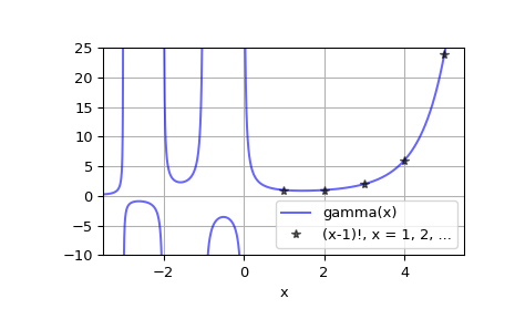
繪製實數 x 的 gamma(x) 圖

>>> x = np.linspace(-3.5, 5.5, 2251)
>>> y = gamma(x)

>>> import matplotlib.pyplot as plt
>>> plt.plot(x, y, 'b', alpha=0.6, label='gamma(x)')
>>> k = np.arange(1, 7)
>>> plt.plot(k, factorial(k-1), 'k*', alpha=0.6,
...          label='(x-1)!, x = 1, 2, ...')
>>> plt.xlim(-3.5, 5.5)
>>> plt.ylim(-10, 25)
>>> plt.grid()
>>> plt.xlabel('x')
>>> plt.legend(loc='lower right')
>>> plt.show()