scipy.special.

chebyu

scipy.special.chebyu(n, monic=False)

第二類切比雪夫多項式。

定義為以下方程式的解

\[(1 - x^2)\frac{d^2}{dx^2}U_n - 3x\frac{d}{dx}U_n + n(n + 2)U_n = 0;\]

\(U_n\) 是 \(n\) 次多項式。

參數:

nint

多項式的次數。

monicbool, optional

若 True，則將前導係數縮放為 1。預設值為 False。

回傳值:

Uorthopoly1d

第二類切比雪夫多項式。

另請參閱

chebyt

第一類切比雪夫多項式。

註解

多項式 \(U_n\) 在 \([-1, 1]\) 區間內對於權重函數 \((1 - x^2)^{1/2}\) 是正交的。

參考文獻

[AS]

Milton Abramowitz 與 Irene A. Stegun (編輯)。Handbook of Mathematical Functions with Formulas, Graphs, and Mathematical Tables。紐約：Dover，1972 年。

範例

在您的瀏覽器中試試看！

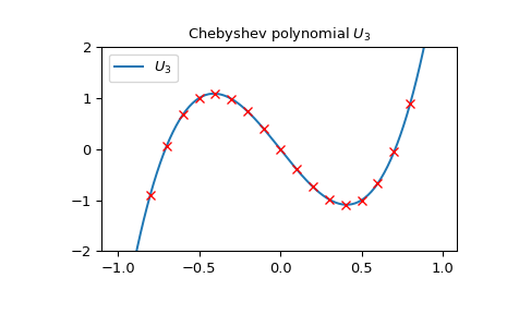
階數為 \(n\) 的第二類切比雪夫多項式可以透過特定 \(n \times n\) 矩陣的行列式獲得。舉例來說，我們可以檢查從以下 \(3 \times 3\) 矩陣的行列式獲得的點如何精確地落在 \(U_3\) 上

>>> import numpy as np
>>> import matplotlib.pyplot as plt
>>> from scipy.linalg import det
>>> from scipy.special import chebyu
>>> x = np.arange(-1.0, 1.0, 0.01)
>>> fig, ax = plt.subplots()
>>> ax.set_ylim(-2.0, 2.0)
>>> ax.set_title(r'Chebyshev polynomial $U_3$')
>>> ax.plot(x, chebyu(3)(x), label=rf'$U_3$')
>>> for p in np.arange(-1.0, 1.0, 0.1):
...     ax.plot(p,
...             det(np.array([[2*p, 1, 0], [1, 2*p, 1], [0, 1, 2*p]])),
...             'rx')
>>> plt.legend(loc='best')
>>> plt.show()

它們滿足遞迴關係式

\[U_{2n-1}(x) = 2 T_n(x)U_{n-1}(x)\]

其中 \(T_n\) 是第一類切比雪夫多項式。讓我們針對 \(n = 2\) 驗證它

>>> from scipy.special import chebyt
>>> x = np.arange(-1.0, 1.0, 0.01)
>>> np.allclose(chebyu(3)(x), 2 * chebyt(2)(x) * chebyu(1)(x))
True

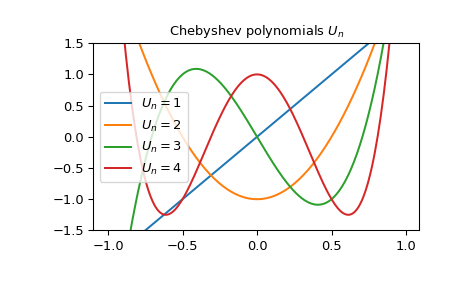
我們可以繪製一些 \(n\) 值的切比雪夫多項式 \(U_n\)

>>> x = np.arange(-1.0, 1.0, 0.01)
>>> fig, ax = plt.subplots()
>>> ax.set_ylim(-1.5, 1.5)
>>> ax.set_title(r'Chebyshev polynomials $U_n$')
>>> for n in np.arange(1,5):
...     ax.plot(x, chebyu(n)(x), label=rf'$U_n={n}$')
>>> plt.legend(loc='best')
>>> plt.show()

返回在新分頁中開啟