scipy.signal.

correlate

scipy.signal.correlate(in1, in2, mode='full', method='auto')

對兩個 N 維陣列進行互相關運算。

對 in1 和 in2 進行互相關運算，輸出大小由 mode 參數決定。

參數:

in1陣列型

第一個輸入。

in2陣列型

第二個輸入。應具有與 in1 相同的維度數。

modestr {‘full’, ‘valid’, ‘same’}, 選填

指示輸出大小的字串

full

輸出是輸入的完整離散線性互相關運算。（預設）

valid

輸出僅包含不依賴零填充的元素。在 'valid' 模式下，in1 或 in2 必須在每個維度上至少與另一個一樣大。

same

輸出與 in1 大小相同，相對於 'full' 輸出居中。

methodstr {‘auto’, ‘direct’, ‘fft’}, 選填

指示用於計算相關性的方法的字串。

direct

相關性直接從總和確定，即相關性的定義。

fft

快速傅立葉變換用於更快速地執行相關運算（僅適用於數值陣列）。

auto

根據哪個更快的估計自動選擇直接或傅立葉方法（預設）。詳情請參閱 convolve 註解。

在版本 0.19.0 中新增。

回傳值:

correlate陣列

一個 N 維陣列，包含 in1 與 in2 的離散線性互相關運算的子集。

另請參閱

choose_conv_method

包含關於 method 的更多文件。

correlation_lags

計算 1D 互相關運算的延遲/位移索引陣列。

註解

兩個 d 維陣列 x 和 y 的相關性 z 定義為

z[...,k,...] = sum[..., i_l, ...] x[..., i_l,...] * conj(y[..., i_l - k,...])

這樣，如果 x 和 y 是 1 維陣列，且 z = correlate(x, y, 'full') 則

\[z[k] = (x * y)(k - N + 1) = \sum_{l=0}^{||x||-1}x_l y_{l-k+N-1}^{*}\]

對於 \(k = 0, 1, ..., ||x|| + ||y|| - 2\)

其中 \(||x||\) 是 x 的長度，\(N = \max(||x||,||y||)\)，且 \(y_m\) 當 m 超出 y 的範圍時為 0。

method='fft' 僅適用於數值陣列，因為它依賴於 fftconvolve。在某些情況下（即，物件陣列或當整數捨入可能損失精度時），始終使用 method='direct'。

當對偶數長度輸入使用 “same” 模式時，correlate 和 correlate2d 的輸出會有所不同：它們之間存在 1 索引偏移。

範例

在您的瀏覽器中試試看！

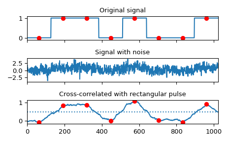
使用互相關運算實作匹配濾波器，以恢復已通過雜訊通道的訊號。

>>> import numpy as np
>>> from scipy import signal
>>> import matplotlib.pyplot as plt
>>> rng = np.random.default_rng()

>>> sig = np.repeat([0., 1., 1., 0., 1., 0., 0., 1.], 128)
>>> sig_noise = sig + rng.standard_normal(len(sig))
>>> corr = signal.correlate(sig_noise, np.ones(128), mode='same') / 128

>>> clock = np.arange(64, len(sig), 128)
>>> fig, (ax_orig, ax_noise, ax_corr) = plt.subplots(3, 1, sharex=True)
>>> ax_orig.plot(sig)
>>> ax_orig.plot(clock, sig[clock], 'ro')
>>> ax_orig.set_title('Original signal')
>>> ax_noise.plot(sig_noise)
>>> ax_noise.set_title('Signal with noise')
>>> ax_corr.plot(corr)
>>> ax_corr.plot(clock, corr[clock], 'ro')
>>> ax_corr.axhline(0.5, ls=':')
>>> ax_corr.set_title('Cross-correlated with rectangular pulse')
>>> ax_orig.margins(0, 0.1)
>>> fig.tight_layout()
>>> plt.show()

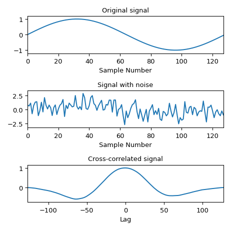
計算雜訊訊號與原始訊號的互相關運算。

>>> x = np.arange(128) / 128
>>> sig = np.sin(2 * np.pi * x)
>>> sig_noise = sig + rng.standard_normal(len(sig))
>>> corr = signal.correlate(sig_noise, sig)
>>> lags = signal.correlation_lags(len(sig), len(sig_noise))
>>> corr /= np.max(corr)

>>> fig, (ax_orig, ax_noise, ax_corr) = plt.subplots(3, 1, figsize=(4.8, 4.8))
>>> ax_orig.plot(sig)
>>> ax_orig.set_title('Original signal')
>>> ax_orig.set_xlabel('Sample Number')
>>> ax_noise.plot(sig_noise)
>>> ax_noise.set_title('Signal with noise')
>>> ax_noise.set_xlabel('Sample Number')
>>> ax_corr.plot(lags, corr)
>>> ax_corr.set_title('Cross-correlated signal')
>>> ax_corr.set_xlabel('Lag')
>>> ax_orig.margins(0, 0.1)
>>> ax_noise.margins(0, 0.1)
>>> ax_corr.margins(0, 0.1)
>>> fig.tight_layout()
>>> plt.show()

返回在新分頁中開啟