scipy.signal.

correlate2d

scipy.signal.correlate2d(in1, in2, mode='full', boundary='fill', fillvalue=0)

對兩個 2 維陣列進行互相關運算。

對 in1 和 in2 進行互相關運算，輸出大小由 mode 決定，邊界條件由 boundary 和 fillvalue 決定。

參數:

in1array_like

第一個輸入。

in2array_like

第二個輸入。應具有與 in1 相同的維度數。

modestr {‘full’, ‘valid’, ‘same’}, optional

指示輸出大小的字串

full

輸出是輸入的完整離散線性互相關。（預設）

valid

輸出僅包含不依賴零填充的元素。在 ‘valid’ 模式下，in1 或 in2 在每個維度上都必須至少與另一個一樣大。

same

輸出與 in1 大小相同，相對於 ‘full’ 輸出居中。

boundarystr {‘fill’, ‘wrap’, ‘symm’}, optional

指示如何處理邊界的旗標

fill

用 fillvalue 填充輸入陣列。（預設）

wrap

循環邊界條件。

symm

對稱邊界條件。

fillvaluescalar, optional

用於填充輸入陣列的值。預設值為 0。

返回:

correlate2dndarray

一個 2 維陣列，包含 in1 與 in2 的離散線性互相關的子集。

註解

當對偶數長度的輸入使用 “same” 模式時，correlate 和 correlate2d 的輸出會有所不同：它們之間存在 1 個索引的偏移。

範例

在您的瀏覽器中試試看！

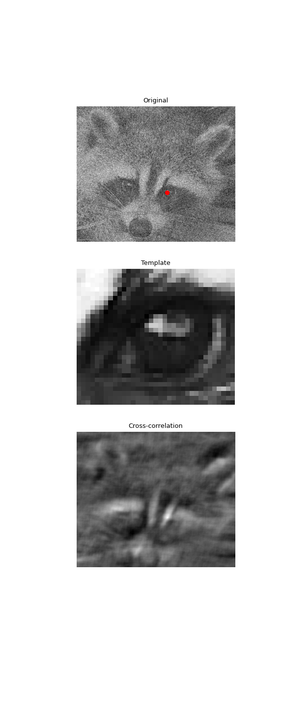
使用 2D 互相關來尋找雜訊影像中範本的位置

>>> import numpy as np
>>> from scipy import signal, datasets, ndimage
>>> rng = np.random.default_rng()
>>> face = datasets.face(gray=True) - datasets.face(gray=True).mean()
>>> face = ndimage.zoom(face[30:500, 400:950], 0.5)  # extract the face
>>> template = np.copy(face[135:165, 140:175])  # right eye
>>> template -= template.mean()
>>> face = face + rng.standard_normal(face.shape) * 50  # add noise
>>> corr = signal.correlate2d(face, template, boundary='symm', mode='same')
>>> y, x = np.unravel_index(np.argmax(corr), corr.shape)  # find the match

>>> import matplotlib.pyplot as plt
>>> fig, (ax_orig, ax_template, ax_corr) = plt.subplots(3, 1,
...                                                     figsize=(6, 15))
>>> ax_orig.imshow(face, cmap='gray')
>>> ax_orig.set_title('Original')
>>> ax_orig.set_axis_off()
>>> ax_template.imshow(template, cmap='gray')
>>> ax_template.set_title('Template')
>>> ax_template.set_axis_off()
>>> ax_corr.imshow(corr, cmap='gray')
>>> ax_corr.set_title('Cross-correlation')
>>> ax_corr.set_axis_off()
>>> ax_orig.plot(x, y, 'ro')
>>> fig.show()

返回在新分頁中開啟