scipy.interpolate.

AAA#

class scipy.interpolate.AAA(x, y, *, rtol=None, max_terms=100, clean_up=True, clean_up_tol=1e-13)[原始碼]#

AAA 實數或複數有理逼近。

如 [1] 所述，AAA 演算法是一種貪婪演算法，用於在實數或複數點集上進行有理函數逼近。有理逼近以重心形式表示，可以從中計算根（零點）、極點和殘差。

參數:

x1D 類陣列，形狀 (n,): 包含自變數值的 1 維陣列。值可以是實數或複數，但必須是有限值。
y1D 類陣列，形狀 (n,): 函數值 f(x)。values 的無限值和 NaN 值，以及 points 的對應值將被捨棄。
rtol浮點數，選填: 相對容差，預設為 eps**0.75。如果 values 中一小部分項遠大於其餘項，則預設容差可能太寬鬆。如果容差太嚴格，則逼近可能包含 Froissart 雙重態，或者演算法可能完全無法收斂。
max_terms整數，選填: 重心表示中的最大項數，預設為 100。必須大於或等於 1。
clean_up布林值，選填: 自動移除 Froissart 雙重態，預設為 True。詳情請參閱註解。
clean_up_tol浮點數，選填: 殘差小於此數字乘以 values 的幾何平均值，再乘以到 points 的最小距離的極點，將被清理程序視為偽造極點，預設為 1e-13。詳情請參閱註解。

警告:

RuntimeWarning: 如果在 max_terms 迭代次數內未達到 rtol。

參見

FloaterHormannInterpolator: Floater-Hormann 重心有理內插。
pade: Padé 逼近。

註解

在迭代 \(m\) 次時（此時逼近的分子和分母中都有 \(m\) 項），AAA 演算法中的有理逼近採用重心形式

\[r(z) = n(z)/d(z) = \frac{\sum_{j=1}^m\ w_j f_j / (z - z_j)}{\sum_{j=1}^m w_j / (z - z_j)},\]

其中 \(z_1,\dots,z_m\) 是從 x 中選取的實數或複數支持點，\(f_1,\dots,f_m\) 是來自 y 的對應實數或複數資料值，而 \(w_1,\dots,w_m\) 是實數或複數權重。

演算法的每次迭代都有兩個部分：貪婪選擇下一個支持點和權重的計算。每次迭代的第一部分是從剩餘未選取的 x 中選擇要新增的下一個支持點 \(z_{m+1}\)，以便最大化非線性殘差 \(|f(z_{m+1}) - n(z_{m+1})/d(z_{m+1})|\)。當此最大值小於 rtol * np.linalg.norm(f, ord=np.inf) 時，演算法終止。這表示內插屬性僅在容差範圍內滿足，但在支持點處，逼近會精確內插提供的資料。

在每次迭代的第二部分中，選擇權重 \(w_j\) 來解決最小平方問題

\[\text{minimise}_{w_j}|fd - n| \quad \text{subject to} \quad \sum_{j=1}^{m+1} w_j = 1,\]

在 x 的未選取元素上。

使用有理逼近的挑戰之一是 Froissart 雙重態的存在，Froissart 雙重態是殘差非常小的極點，或是足夠接近以至於幾乎抵消的極點-零點對，請參閱 [2]。AAA 演算法的貪婪性質表示 Froissart 雙重態很少見。但是，如果 rtol 設定得太嚴格，則逼近將停滯，並且會出現許多 Froissart 雙重態。Froissart 雙重態通常可以通過移除支持點，然後重新解決最小平方問題來移除。如果滿足以下條件，則移除支持點 \(z_j\)，它是最接近殘差為 \(\alpha\) 的極點 \(a\) 的支持點

\[|\alpha| / |z_j - a| < \verb|clean_up_tol| \cdot \tilde{f},\]

其中 \(\tilde{f}\) 是 support_values 的幾何平均值。

參考文獻

[1] (1,2,3)

Y. Nakatsukasa、O. Sete 和 L. N. Trefethen，“The AAA algorithm for rational approximation”，SIAM J. Sci. Comp. 40 (2018)，A1494-A1522。 DOI:10.1137/16M1106122

[2]

J. Gilewicz 和 M. Pindor，Pade approximants and noise: rational functions，J. Comp. Appl. Math. 105 (1999)，pp. 285-297。 DOI:10.1016/S0377-0427(02)00674-X

範例

這裡我們重現了許多來自 [1] 的數值範例，以示範此方法提供的功能。

>>> import numpy as np
>>> import matplotlib.pyplot as plt
>>> from scipy.interpolate import AAA
>>> import warnings

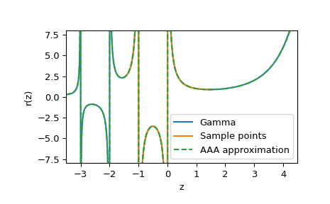
在第一個範例中，我們通過從 [-1.5, 1.5] 中的 100 個樣本外插，來逼近 [-3.5, 4.5] 上的伽瑪函數。

>>> from scipy.special import gamma
>>> sample_points = np.linspace(-1.5, 1.5, num=100)
>>> r = AAA(sample_points, gamma(sample_points))
>>> z = np.linspace(-3.5, 4.5, num=1000)
>>> fig, ax = plt.subplots()
>>> ax.plot(z, gamma(z), label="Gamma")
>>> ax.plot(sample_points, gamma(sample_points), label="Sample points")
>>> ax.plot(z, r(z).real, '--', label="AAA approximation")
>>> ax.set(xlabel="z", ylabel="r(z)", ylim=[-8, 8], xlim=[-3.5, 4.5])
>>> ax.legend()
>>> plt.show()

../../_images/scipy-interpolate-AAA-1_00_00.png

我們還可以查看有理逼近的極點及其殘差

>>> order = np.argsort(r.poles())
>>> r.poles()[order]
array([-3.81591039e+00+0.j        , -3.00269049e+00+0.j        ,
       -1.99999988e+00+0.j        , -1.00000000e+00+0.j        ,
        5.85842812e-17+0.j        ,  4.77485458e+00-3.06919376j,
        4.77485458e+00+3.06919376j,  5.29095868e+00-0.97373072j,
        5.29095868e+00+0.97373072j])
>>> r.residues()[order]
array([ 0.03658074 +0.j        , -0.16915426 -0.j        ,
        0.49999915 +0.j        , -1.         +0.j        ,
        1.         +0.j        , -0.81132013 -2.30193429j,
       -0.81132013 +2.30193429j,  0.87326839+10.70148546j,
        0.87326839-10.70148546j])

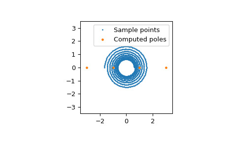
在第二個範例中，我們使用在複數平面中繞原點旋轉 7.5 圈的 1000 個點的螺旋來呼叫 AAA。

>>> z = np.exp(np.linspace(-0.5, 0.5 + 15j*np.pi, 1000))
>>> r = AAA(z, np.tan(np.pi*z/2), rtol=1e-13)

我們看到 AAA 經過 12 個步驟收斂，誤差如下

>>> r.errors.size
12
>>> r.errors
array([2.49261500e+01, 4.28045609e+01, 1.71346935e+01, 8.65055336e-02,
       1.27106444e-02, 9.90889874e-04, 5.86910543e-05, 1.28735561e-06,
       3.57007424e-08, 6.37007837e-10, 1.67103357e-11, 1.17112299e-13])

我們還可以繪製計算出的極點

>>> fig, ax = plt.subplots()
>>> ax.plot(z.real, z.imag, '.', markersize=2, label="Sample points")
>>> ax.plot(r.poles().real, r.poles().imag, '.', markersize=5,
...         label="Computed poles")
>>> ax.set(xlim=[-3.5, 3.5], ylim=[-3.5, 3.5], aspect="equal")
>>> ax.legend()
>>> plt.show()

../../_images/scipy-interpolate-AAA-1_01_00.png

現在，我們使用來自 [1] 的範例，示範如何使用 clean_up 方法移除 Froissart 雙重態。此演算法在 rtol=0 和 clean_up=False 的情況下執行，以刻意產生 Froissart 雙重態。

>>> z = np.exp(1j*2*np.pi*np.linspace(0,1, num=1000))
>>> def f(z):
...     return np.log(2 + z**4)/(1 - 16*z**4)
>>> with warnings.catch_warnings():  # filter convergence warning due to rtol=0
...     warnings.simplefilter('ignore', RuntimeWarning)
...     r = AAA(z, f(z), rtol=0, max_terms=50, clean_up=False)
>>> mask = np.abs(r.residues()) < 1e-13
>>> fig, axs = plt.subplots(ncols=2)
>>> axs[0].plot(r.poles().real[~mask], r.poles().imag[~mask], '.')
>>> axs[0].plot(r.poles().real[mask], r.poles().imag[mask], 'r.')

現在我們呼叫 clean_up 方法來移除 Froissart 雙重態。

>>> with warnings.catch_warnings():
...     warnings.simplefilter('ignore', RuntimeWarning)
...     r.clean_up()
4
>>> mask = np.abs(r.residues()) < 1e-13
>>> axs[1].plot(r.poles().real[~mask], r.poles().imag[~mask], '.')
>>> axs[1].plot(r.poles().real[mask], r.poles().imag[mask], 'r.')
>>> plt.show()

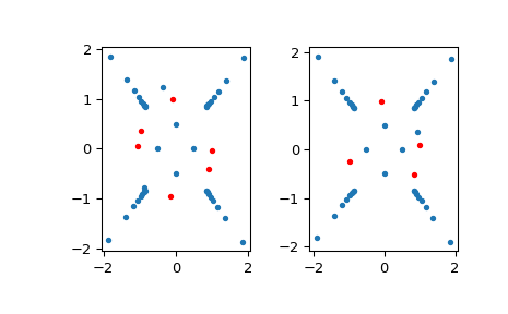
../../_images/scipy-interpolate-AAA-1_02_00.png

左圖顯示了逼近 clean_up=False 之前的極點，絕對值小於 10^-13 的殘差的極點以紅色顯示。右圖顯示了呼叫 clean_up 方法後的極點。

屬性:

support_points陣列: 逼近的支持點。這些是提供的 x 的子集，逼近在此子集處嚴格內插 y。詳情請參閱註解。
support_values陣列: 逼近在 support_points 處的值。
weights陣列: 重心逼近的權重。
errors陣列: AAA 的連續迭代中，points 上的誤差 \(|f(z) - r(z)|_\infty\)。

方法

`__call__`(z)	在給定值下評估有理逼近。
`clean_up`([cleanup_tol])	自動移除 Froissart 雙重態。
`poles`()	計算有理逼近的極點。
`residues`()	計算逼近極點的殘差。
`roots`()	計算有理逼近的零點。