theilslopes#
- scipy.stats.theilslopes(y, x=None, alpha=0.95, method='separate')[原始碼]#
計算一組點 (x, y) 的 Theil-Sen 估計量。
theilslopes實作了一種穩健線性迴歸的方法。它將斜率計算為成對值之間所有斜率的中位數。- 參數:
- yarray_like
應變數。
- xarray_like 或 None,可選
自變數。如果為 None,則改用
arange(len(y))。- alphafloat,可選
介於 0 和 1 之間的信賴度。預設值為 95% 信賴度。請注意,
alpha以 0.5 為中心對稱,即 0.1 和 0.9 都被解釋為「找到 90% 信賴區間」。- method{‘joint’, ‘separate’},可選
用於計算截距估計值的方法。支援以下方法,
‘joint’:使用 np.median(y - slope * x) 作為截距。
- ‘separate’:使用 np.median(y) - slope * np.median(x)
作為截距。
預設值為 ‘separate’。
在 1.8.0 版本中新增。
- 回傳:
- result
TheilslopesResult實例 回傳值是一個具有以下屬性的物件
- slopefloat
Theil 斜率。
- interceptfloat
Theil 線的截距。
- low_slopefloat
斜率 slope 的信賴區間下限。
- high_slopefloat
斜率 slope 的信賴區間上限。
- result
另請參閱
siegelslopes一種使用重複中位數的類似技術
註解
theilslopes的實作遵循 [1]。[1] 中未定義截距,此處定義為median(y) - slope*median(x),這在 [3] 中給出。文獻中存在截距的其他定義,例如median(y - slope*x)在 [4] 中。可以通過參數method確定計算截距的方法。由於 [1] 中未解決此問題,因此未給出截距的信賴區間。為了與舊版本的 SciPy 相容,回傳值的行為類似於長度為 4 的
namedtuple,欄位為slope、intercept、low_slope和high_slope,因此可以繼續寫入slope, intercept, low_slope, high_slope = theilslopes(y, x)
參考文獻
[1] (1,2,3)P.K. Sen, “Estimates of the regression coefficient based on Kendall’s tau”, J. Am. Stat. Assoc., Vol. 63, pp. 1379-1389, 1968.
[2]H. Theil, “A rank-invariant method of linear and polynomial regression analysis I, II and III”, Nederl. Akad. Wetensch., Proc. 53:, pp. 386-392, pp. 521-525, pp. 1397-1412, 1950.
[3]W.L. Conover, “Practical nonparametric statistics”, 2nd ed., John Wiley and Sons, New York, pp. 493.
範例
>>> import numpy as np
>>> from scipy import stats
>>> import matplotlib.pyplot as plt
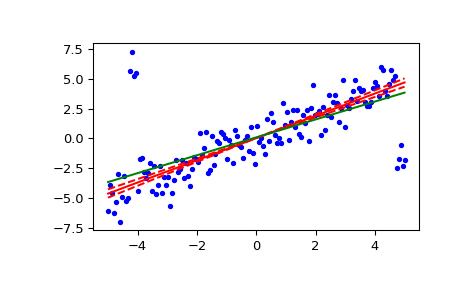
>>> x = np.linspace(-5, 5, num=150)
>>> y = x + np.random.normal(size=x.size)
>>> y[11:15] += 10  # add outliers
>>> y[-5:] -= 7
計算斜率、截距和 90% 信賴區間。為了比較,也使用
linregress計算最小平方法擬合>>> res = stats.theilslopes(y, x, 0.90, method='separate') >>> lsq_res = stats.linregress(x, y)
繪製結果。Theil-Sen 迴歸線以紅色顯示,虛線紅線表示斜率的信賴區間(請注意,虛線紅線不是迴歸的信賴區間,因為未包含截距的信賴區間)。綠線顯示最小平方法擬合以供比較。
>>> fig = plt.figure()
>>> ax = fig.add_subplot(111)
>>> ax.plot(x, y, 'b.')
>>> ax.plot(x, res[1] + res[0] * x, 'r-')
>>> ax.plot(x, res[1] + res[2] * x, 'r--')
>>> ax.plot(x, res[1] + res[3] * x, 'r--')
>>> ax.plot(x, lsq_res[1] + lsq_res[0] * x, 'g-')
>>> plt.show()