scipy.stats.mielke#
- scipy.stats.mielke = <scipy.stats._continuous_distns.mielke_gen object>[source]#
Mielke Beta-Kappa / Dagum 連續隨機變數。
作為
rv_continuous類別的一個實例,mielke物件繼承了它的一系列通用方法(完整列表請見下方),並針對此特定分佈補充了詳細資訊。說明
mielke的機率密度函數為\[f(x, k, s) = \frac{k x^{k-1}}{(1+x^s)^{1+k/s}}\]針對 \(x > 0\) 且 \(k, s > 0\)。此分佈有時稱為 Dagum 分佈 ([2])。它已在 [3] 中定義,稱為 Burr III 型分佈 (
burr參數為c=s和d=k/s)。mielke接受k和s作為形狀參數。上述機率密度以「標準化」形式定義。若要移動和/或縮放分佈,請使用
loc和scale參數。具體而言,mielke.pdf(x, k, s, loc, scale)與mielke.pdf(y, k, s) / scale完全等效,其中y = (x - loc) / scale。請注意,移動分佈的位置不會使其成為「非中心」分佈;某些分佈的非中心廣義化版本在不同的類別中提供。參考文獻
[1]Mielke, P.W., 1973 “Another Family of Distributions for Describing and Analyzing Precipitation Data.” J. Appl. Meteor., 12, 275-280
[2]Dagum, C., 1977 “A new model for personal income distribution.” Economie Appliquee, 33, 327-367.
[3]Burr, I. W. “Cumulative frequency functions”, Annals of Mathematical Statistics, 13(2), pp 215-232 (1942).
範例
>>> import numpy as np
>>> from scipy.stats import mielke
>>> import matplotlib.pyplot as plt
>>> fig, ax = plt.subplots(1, 1)
計算前四個動差
>>> k, s = 10.4, 4.6
>>> mean, var, skew, kurt = mielke.stats(k, s, moments='mvsk')
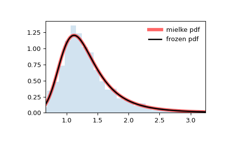
顯示機率密度函數 (
pdf)>>> x = np.linspace(mielke.ppf(0.01, k, s), ... mielke.ppf(0.99, k, s), 100) >>> ax.plot(x, mielke.pdf(x, k, s), ... 'r-', lw=5, alpha=0.6, label='mielke pdf')
或者,可以呼叫分佈物件(作為函數)來固定形狀、位置和尺度參數。這會傳回一個「凍結」的 RV 物件,其中保存了給定的固定參數。
凍結分佈並顯示凍結的
pdf>>> rv = mielke(k, s) >>> ax.plot(x, rv.pdf(x), 'k-', lw=2, label='frozen pdf')
檢查
cdf和ppf的準確性>>> vals = mielke.ppf([0.001, 0.5, 0.999], k, s) >>> np.allclose([0.001, 0.5, 0.999], mielke.cdf(vals, k, s)) True
產生隨機數字
>>> r = mielke.rvs(k, s, size=1000)
並比較直方圖
>>> ax.hist(r, density=True, bins='auto', histtype='stepfilled', alpha=0.2)
>>> ax.set_xlim([x[0], x[-1]])
>>> ax.legend(loc='best', frameon=False)
>>> plt.show()
方法
rvs(k, s, loc=0, scale=1, size=1, random_state=None)
隨機變量。
pdf(x, k, s, loc=0, scale=1)
機率密度函數。
logpdf(x, k, s, loc=0, scale=1)
機率密度函數的對數。
cdf(x, k, s, loc=0, scale=1)
累積分布函數。
logcdf(x, k, s, loc=0, scale=1)
累積分布函數的對數。
sf(x, k, s, loc=0, scale=1)
生存函數(也定義為
1 - cdf,但 sf 有時更準確)。logsf(x, k, s, loc=0, scale=1)
生存函數的對數。
ppf(q, k, s, loc=0, scale=1)
百分點函數(
cdf的反函數 — 百分位數)。isf(q, k, s, loc=0, scale=1)
反向生存函數(
sf的反函數)。moment(order, k, s, loc=0, scale=1)
指定階數的非中心動差。
stats(k, s, loc=0, scale=1, moments=’mv’)
平均值 ('m')、變異數 ('v')、偏度 ('s') 和/或峰度 ('k')。
entropy(k, s, loc=0, scale=1)
RV 的(微分)熵。
fit(data)
通用資料的參數估計。有關關鍵字引數的詳細文件,請參閱 scipy.stats.rv_continuous.fit。
expect(func, args=(k, s), loc=0, scale=1, lb=None, ub=None, conditional=False, **kwds)
函數(一個引數)相對於分佈的期望值。
median(k, s, loc=0, scale=1)
分佈的中位數。
mean(k, s, loc=0, scale=1)
分佈的平均值。
var(k, s, loc=0, scale=1)
分佈的變異數。
std(k, s, loc=0, scale=1)
分佈的標準差。
interval(confidence, k, s, loc=0, scale=1)
中位數周圍等面積的信賴區間。