scipy.stats.landau#

scipy.stats.landau = <scipy.stats._continuous_distns.landau_gen object>[原始碼]#

Landau 連續隨機變數。

作為 rv_continuous 類別的實例，landau 物件繼承了其通用方法集合（完整列表請見下方），並以針對此特定分佈的詳細資訊加以完善。

筆記

對於 landau 的機率密度函數 ([1], [2]) 為

\[f(x) = \frac{1}{\pi}\int_0^\infty \exp(-t \log t - xt)\sin(\pi t) dt\]

對於實數 \(x\)。

上面的機率密度是以「標準化」形式定義的。若要位移和/或縮放分佈，請使用 loc 和 scale 參數。具體而言，landau.pdf(x, loc, scale) 與 landau.pdf(y) / scale 完全等效，其中 y = (x - loc) / scale。請注意，移動分佈的位置並不會使其成為「非中心」分佈；某些分佈的非中心廣義化版本在單獨的類別中提供。

通常（例如 [2]），Landau 分佈以位置參數 \(\mu\) 和尺度參數 \(c\) 表示參數，後者也引入了位置位移。如果 mu 和 c 用於表示這些參數，則這與 SciPy 的參數化相對應，其中 loc = mu + 2*c / np.pi * np.log(c) 和 scale = c。

此分佈使用 Boost Math C++ 函式庫中的常式來計算 pdf、cdf、ppf、sf 和 isf 方法。 [1]

參考文獻

[1] (1,2)

Landau, L. (1944). “On the energy loss of fast particles by ionization”. J. Phys. (USSR). 8: 201.

[2] (1,2)

“Landau Distribution”, Wikipedia, https://en.wikipedia.org/wiki/Landau_distribution

[3]

Chambers, J. M., Mallows, C. L., & Stuck, B. (1976). “A method for simulating stable random variables.” Journal of the American Statistical Association, 71(354), 340-344.

[4]

The Boost Developers. “Boost C++ Libraries”. https://boost.dev.org.tw/.

[5]

Yoshimura, T. “Numerical Evaluation and High Precision Approximation Formula for Landau Distribution”. DOI:10.36227/techrxiv.171822215.53612870/v2

範例

>>> import numpy as np
>>> from scipy.stats import landau
>>> import matplotlib.pyplot as plt
>>> fig, ax = plt.subplots(1, 1)

計算前四個動差

>>> mean, var, skew, kurt = landau.stats(moments='mvsk')

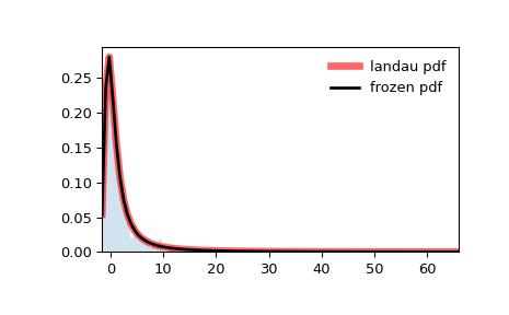
顯示機率密度函數 (pdf)

>>> x = np.linspace(landau.ppf(0.01),
...                 landau.ppf(0.99), 100)
>>> ax.plot(x, landau.pdf(x),
...        'r-', lw=5, alpha=0.6, label='landau pdf')

或者，可以呼叫分佈物件（作為函數）來固定形狀、位置和尺度參數。這會傳回一個「凍結」的 RV 物件，其中保存了給定的固定參數。

凍結分佈並顯示凍結的 pdf

>>> rv = landau()
>>> ax.plot(x, rv.pdf(x), 'k-', lw=2, label='frozen pdf')

檢查 cdf 和 ppf 的準確性

>>> vals = landau.ppf([0.001, 0.5, 0.999])
>>> np.allclose([0.001, 0.5, 0.999], landau.cdf(vals))
True

產生隨機數字

>>> r = landau.rvs(size=1000)

並比較直方圖

>>> ax.hist(r, density=True, bins='auto', histtype='stepfilled', alpha=0.2)
>>> ax.set_xlim([x[0], x[-1]])
>>> ax.legend(loc='best', frameon=False)
>>> plt.show()

方法

rvs(loc=0, scale=1, size=1, random_state=None)	隨機變量。
pdf(x, loc=0, scale=1)	機率密度函數。
logpdf(x, loc=0, scale=1)	機率密度函數的對數。
cdf(x, loc=0, scale=1)	累積分布函數。
logcdf(x, loc=0, scale=1)	累積分布函數的對數。
sf(x, loc=0, scale=1)	生存函數（也定義為 `1 - cdf`，但 sf 有時更準確）。
logsf(x, loc=0, scale=1)	生存函數的對數。
ppf(q, loc=0, scale=1)	百分點函數（`cdf` 的反函數 — 百分位數）。
isf(q, loc=0, scale=1)	反生存函數（`sf` 的反函數）。
moment(order, loc=0, scale=1)	指定階數的非中心動差。
stats(loc=0, scale=1, moments=’mv’)	平均值 ('m')、變異數 ('v')、偏度 ('s') 和/或峰度 ('k')。
entropy(loc=0, scale=1)	RV 的（微分）熵。
fit(data)	通用資料的參數估計。有關關鍵字引數的詳細文件，請參閱 scipy.stats.rv_continuous.fit。
expect(func, args=(), loc=0, scale=1, lb=None, ub=None, conditional=False, kwds)**	函數（一個引數）關於分佈的期望值。
median(loc=0, scale=1)	分佈的中位數。
mean(loc=0, scale=1)	分佈的平均值。
var(loc=0, scale=1)	分佈的變異數。
std(loc=0, scale=1)	分佈的標準差。
interval(confidence, loc=0, scale=1)	具有圍繞中位數的相等區域的信賴區間。