scipy.stats.argus

scipy.stats.argus = <scipy.stats._continuous_distns.argus_gen object>

Argus 分布

作為 rv_continuous 類別的一個實例，argus 物件繼承了它的一系列通用方法（完整列表請見下方），並以針對此特定分布的詳細資訊加以完善。

註解

argus 的機率密度函數為

\[f(x, \chi) = \frac{\chi^3}{\sqrt{2\pi} \Psi(\chi)} x \sqrt{1-x^2} \exp(-\chi^2 (1 - x^2)/2)\]

針對 \(0 < x < 1\) 且 \(\chi > 0\)，其中

\[\Psi(\chi) = \Phi(\chi) - \chi \phi(\chi) - 1/2\]

其中 \(\Phi\) 和 \(\phi\) 分別為標準常態分布的 CDF 和 PDF。

argus 接受 \(\chi\) 作為形狀參數。關於從 ARGUS 分布取樣的詳細資訊，請參閱 [2]。

上述機率密度是以「標準化」形式定義的。若要平移和/或縮放分布，請使用 loc 和 scale 參數。具體來說，argus.pdf(x, chi, loc, scale) 與 argus.pdf(y, chi) / scale 完全等效，其中 y = (x - loc) / scale。請注意，平移分布的位置不會使其成為「非中心」分布；某些分布的非中心廣義化版本可在個別的類別中找到。

參考文獻

[1]

“ARGUS distribution”, https://en.wikipedia.org/wiki/ARGUS_distribution

[2]

Christoph Baumgarten “Random variate generation by fast numerical inversion in the varying parameter case.” Research in Statistics, vol. 1, 2023, doi:10.1080/27684520.2023.2279060.

於版本 0.19.0 中新增。

範例

在您的瀏覽器中試試看！

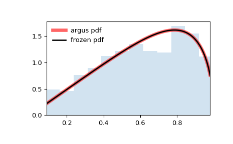
>>> import numpy as np
>>> from scipy.stats import argus
>>> import matplotlib.pyplot as plt
>>> fig, ax = plt.subplots(1, 1)

計算前四個動差

>>> chi = 1
>>> mean, var, skew, kurt = argus.stats(chi, moments='mvsk')

顯示機率密度函數 (pdf)

>>> x = np.linspace(argus.ppf(0.01, chi),
...                 argus.ppf(0.99, chi), 100)
>>> ax.plot(x, argus.pdf(x, chi),
...        'r-', lw=5, alpha=0.6, label='argus pdf')

或者，可以呼叫分布物件（作為函數）以固定形狀、位置和尺度參數。這會傳回一個「凍結的」RV 物件，其中保存了給定的固定參數。

凍結分布並顯示凍結的 pdf

>>> rv = argus(chi)
>>> ax.plot(x, rv.pdf(x), 'k-', lw=2, label='frozen pdf')

檢查 cdf 和 ppf 的準確性

>>> vals = argus.ppf([0.001, 0.5, 0.999], chi)
>>> np.allclose([0.001, 0.5, 0.999], argus.cdf(vals, chi))
True

產生隨機數字

>>> r = argus.rvs(chi, size=1000)

並比較直方圖

>>> ax.hist(r, density=True, bins='auto', histtype='stepfilled', alpha=0.2)
>>> ax.set_xlim([x[0], x[-1]])
>>> ax.legend(loc='best', frameon=False)
>>> plt.show()

返回在新分頁中開啟

方法

rvs(chi, loc=0, scale=1, size=1, random_state=None)	隨機變量。
pdf(x, chi, loc=0, scale=1)	機率密度函數。
logpdf(x, chi, loc=0, scale=1)	機率密度函數的對數。
cdf(x, chi, loc=0, scale=1)	累積分布函數。
logcdf(x, chi, loc=0, scale=1)	累積分布函數的對數。
sf(x, chi, loc=0, scale=1)	存活函數（也定義為 1 - cdf，但 sf 有時更準確）。
logsf(x, chi, loc=0, scale=1)	存活函數的對數。
ppf(q, chi, loc=0, scale=1)	百分點函數（cdf 的反函數 — 百分位數）。
isf(q, chi, loc=0, scale=1)	反向存活函數（sf 的反函數）。
moment(order, chi, loc=0, scale=1)	指定階數的非中心動差。
stats(chi, loc=0, scale=1, moments=’mv’)	平均值 ('m')、變異數 ('v')、偏度 ('s') 和/或峰度 ('k')。
entropy(chi, loc=0, scale=1)	RV 的（微分）熵。
fit(data)	通用資料的參數估計。 有關關鍵字引數的詳細文件，請參閱 scipy.stats.rv_continuous.fit。
expect(func, args=(chi,), loc=0, scale=1, lb=None, ub=None, conditional=False, **kwds)	函數（一個引數）相對於分布的期望值。
median(chi, loc=0, scale=1)	分布的中位數。
mean(chi, loc=0, scale=1)	分布的平均值。
var(chi, loc=0, scale=1)	分布的變異數。
std(chi, loc=0, scale=1)	分布的標準差。
interval(confidence, chi, loc=0, scale=1)	中位數周圍等面積的信賴區間。