scipy.special.struve#
- scipy.special.struve(v, x, out=None) = <ufunc 'struve'>#
Struve 函數。
返回階數為 v,自變數為 x 的 Struve 函數值。Struve 函數定義如下:
\[H_v(x) = (z/2)^{v + 1} \sum_{n=0}^\infty \frac{(-1)^n (z/2)^{2n}}{\Gamma(n + \frac{3}{2}) \Gamma(n + v + \frac{3}{2})},\]其中 \(\Gamma\) 是 gamma 函數。
- 參數:
- varray_like
Struve 函數的階數 (浮點數)。
- xarray_like
Struve 函數的自變數 (浮點數;除非 v 是整數,否則必須為正數)。
- outndarray, optional
函數結果的選用性輸出陣列
- 返回:
- Hscalar or ndarray
階數為 v,自變數為 x 的 Struve 函數值。
參見
modstruve修正的 Struve 函數
註解
文獻 [1] 中討論了三種用於評估 Struve 函數的方法
冪級數
貝索函數展開式 (如果 \(|z| < |v| + 20\))
大自變數 z 的漸近展開式 (如果 \(z \geq 0.7v + 12\))
捨入誤差是根據總和中最大的項估算的,並返回與最小誤差相關聯的結果。
參考文獻
[1]NIST 數學函數數位圖書館 https://dlmf.nist.gov/11
範例
計算階數為 1,自變數為 2 的 Struve 函數。
>>> import numpy as np
>>> from scipy.special import struve
>>> import matplotlib.pyplot as plt
>>> struve(1, 2.)
0.6467637282835622
透過為階數參數 v 提供列表,計算自變數為 2,階數分別為 1、2 和 3 的 Struve 函數。
>>> struve([1, 2, 3], 2.)
array([0.64676373, 0.28031806, 0.08363767])
透過為 x 提供陣列,計算階數為 1 的 Struve 函數在多個點的值。
>>> points = np.array([2., 5., 8.])
>>> struve(1, points)
array([0.64676373, 0.80781195, 0.48811605])
透過為 v 和 x 提供陣列,計算多個階數在多個點的 Struve 函數。陣列必須可廣播為正確的形狀。
>>> orders = np.array([[1], [2], [3]])
>>> points.shape, orders.shape
((3,), (3, 1))
>>> struve(orders, points)
array([[0.64676373, 0.80781195, 0.48811605],
       [0.28031806, 1.56937455, 1.51769363],
       [0.08363767, 1.50872065, 2.98697513]])
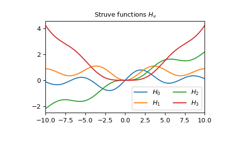
繪製階數從 0 到 3,範圍從 -10 到 10 的 Struve 函數圖。
>>> fig, ax = plt.subplots()
>>> x = np.linspace(-10., 10., 1000)
>>> for i in range(4):
...     ax.plot(x, struve(i, x), label=f'$H_{i!r}$')
>>> ax.legend(ncol=2)
>>> ax.set_xlim(-10, 10)
>>> ax.set_title(r"Struve functions $H_{\nu}$")
>>> plt.show()