scipy.special.it2i0k0

scipy.special.it2i0k0(x, out=None) = <ufunc 'it2i0k0'>

與 0 階修正貝塞爾函數相關的積分。

計算積分

\[\begin{split}\int_0^x \frac{I_0(t) - 1}{t} dt \\ \int_x^\infty \frac{K_0(t)}{t} dt.\end{split}\]

參數:

xarray_like

評估積分的值。

outtuple of ndarrays, optional

函數結果的可選輸出陣列。

返回:

ii0scalar or ndarray

i0 的積分

ik0scalar or ndarray

k0 的積分

參考文獻

[1]

S. Zhang and J.M. Jin, “Computation of Special Functions”, Wiley 1996

範例

在您的瀏覽器中試試看！

在一個點評估函數。

>>> from scipy.special import it2i0k0
>>> int_i, int_k = it2i0k0(1.)
>>> int_i, int_k
(0.12897944249456852, 0.2085182909001295)

在多個點評估函數。

>>> import numpy as np
>>> points = np.array([0.5, 1.5, 3.])
>>> int_i, int_k = it2i0k0(points)
>>> int_i, int_k
(array([0.03149527, 0.30187149, 1.50012461]),
 array([0.66575102, 0.0823715 , 0.00823631]))

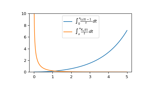
繪製從 0 到 5 的函數圖。

>>> import matplotlib.pyplot as plt
>>> fig, ax = plt.subplots()
>>> x = np.linspace(0., 5., 1000)
>>> int_i, int_k = it2i0k0(x)
>>> ax.plot(x, int_i, label=r"$\int_0^x \frac{I_0(t)-1}{t}\,dt$")
>>> ax.plot(x, int_k, label=r"$\int_x^{\infty} \frac{K_0(t)}{t}\,dt$")
>>> ax.legend()
>>> ax.set_ylim(0, 10)
>>> plt.show()

返回在新分頁中開啟