chirp#
- scipy.signal.chirp(t, f0, t1, f1, method='linear', phi=0, vertex_zero=True, *, complex=False)[source]#
頻率掃描餘弦波產生器。
在以下內容中,「Hz」應被理解為「每單位週期」;此處不要求單位為一秒。重要的區別在於旋轉的單位是週期,而不是弧度。同樣地,t 可以是空間而不是時間的量測。
- 參數:
- tarray_like
評估波形的 সময় 間點。
- f0float
在時間 t=0 時的頻率(例如 Hz)。
- t1float
指定 f1 的時間點。
- f1float
在時間 t1 時的波形頻率(例如 Hz)。
- method{‘linear’, ‘quadratic’, ‘logarithmic’, ‘hyperbolic’}, optional
頻率掃描的種類。如果未給定,則假定為 linear。詳情請參閱下面的註釋。
- phifloat, optional
相位偏移,以度為單位。預設值為 0。
- vertex_zerobool, optional
此參數僅在 method 為 ‘quadratic’ 時使用。它決定了頻率圖形的拋物線頂點是在 t=0 還是 t=t1。
- complexbool, optional
此參數建立複數值的解析訊號,而不是實數值的訊號。它允許使用複數基頻(在通訊領域中)。預設值為 False。
在 1.15.0 版本中新增。
- 返回:
- yndarray
一個 NumPy 陣列,包含在 t 處評估的訊號,具有請求的隨時間變化的頻率。更精確地說,該函數返回
exp(1j*phase + 1j*(pi/180)*phi) if complex else cos(phase + (pi/180)*phi),其中 phase 是2*pi*f(t)從 0 到 t 的積分。瞬時頻率f(t)定義如下。
另請參閱
註釋
參數 method 有四種可能的選項,它們具有(長的)標準形式和一些允許的縮寫。產生訊號的瞬時頻率 \(f(t)\) 的公式如下
參數 method 在
('linear', 'lin', 'li')中\[f(t) = f_0 + \beta\, t \quad\text{with}\quad \beta = \frac{f_1 - f_0}{t_1}\]頻率 \(f(t)\) 隨時間線性變化,變化率 \(\beta\) 恆定。
參數 method 在
('quadratic', 'quad', 'q')中\[\begin{split}f(t) = \begin{cases} f_0 + \beta\, t^2 & \text{if vertex_zero is True,}\\ f_1 + \beta\, (t_1 - t)^2 & \text{otherwise,} \end{cases} \quad\text{with}\quad \beta = \frac{f_1 - f_0}{t_1^2}\end{split}\]頻率 f(t) 的圖形是通過 \((0, f_0)\) 和 \((t_1, f_1)\) 的拋物線。預設情況下,拋物線的頂點在 \((0, f_0)\)。如果 vertex_zero 為
False,則頂點在 \((t_1, f_1)\)。要使用更一般的二次函數或任意多項式,請使用函數scipy.signal.sweep_poly。參數 method 在
('logarithmic', 'log', 'lo')中\[f(t) = f_0 \left(\frac{f_1}{f_0}\right)^{t/t_1}\]\(f_0\) 和 \(f_1\) 必須是非零值且具有相同的符號。此訊號也稱為幾何或指數啁啾。
參數 method 在
('hyperbolic', 'hyp')中\[f(t) = \frac{\alpha}{\beta\, t + \gamma} \quad\text{with}\quad \alpha = f_0 f_1 t_1, \ \beta = f_0 - f_1, \ \gamma = f_1 t_1\]\(f_0\) 和 \(f_1\) 必須是非零值。
範例
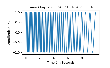
對於第一個範例,繪製了在 10 秒內從 6 Hz 到 1 Hz 的線性啁啾
>>> import numpy as np
>>> from matplotlib.pyplot import tight_layout
>>> from scipy.signal import chirp, square, ShortTimeFFT
>>> from scipy.signal.windows import gaussian
>>> import matplotlib.pyplot as plt
...
>>> N, T = 1000, 0.01  # number of samples and sampling interval for 10 s signal
>>> t = np.arange(N) * T  # timestamps
...
>>> x_lin = chirp(t, f0=6, f1=1, t1=10, method='linear')
...
>>> fg0, ax0 = plt.subplots()
>>> ax0.set_title(r"Linear Chirp from $f(0)=6\,$Hz to $f(10)=1\,$Hz")
>>> ax0.set(xlabel="Time $t$ in Seconds", ylabel=r"Amplitude $x_\text{lin}(t)$")
>>> ax0.plot(t, x_lin)
>>> plt.show()
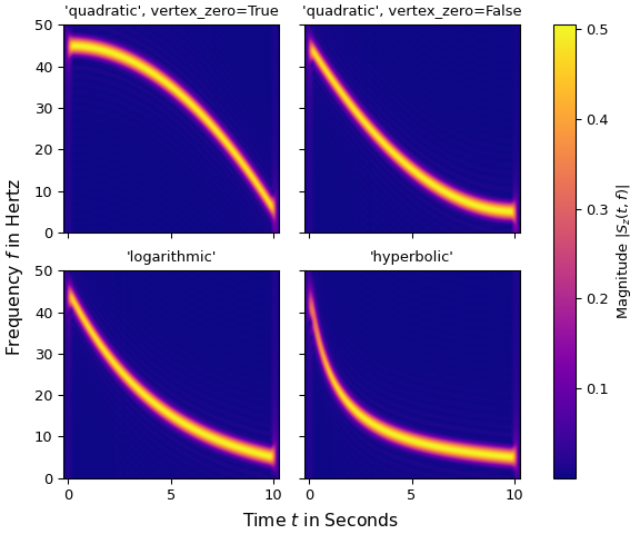
以下四個圖表分別顯示了從 45 Hz 到 5 Hz 的啁啾的短時傅立葉變換,參數 method(和 vertex_zero)使用不同的值
>>> x_qu0 = chirp(t, f0=45, f1=5, t1=N*T, method='quadratic', vertex_zero=True)
>>> x_qu1 = chirp(t, f0=45, f1=5, t1=N*T, method='quadratic', vertex_zero=False)
>>> x_log = chirp(t, f0=45, f1=5, t1=N*T, method='logarithmic')
>>> x_hyp = chirp(t, f0=45, f1=5, t1=N*T, method='hyperbolic')
...
>>> win = gaussian(50, std=12, sym=True)
>>> SFT = ShortTimeFFT(win, hop=2, fs=1/T, mfft=800, scale_to='magnitude')
>>> ts = ("'quadratic', vertex_zero=True", "'quadratic', vertex_zero=False",
...       "'logarithmic'", "'hyperbolic'")
>>> fg1, ax1s = plt.subplots(2, 2, sharex='all', sharey='all',
...                          figsize=(6, 5),  layout="constrained")
>>> for x_, ax_, t_ in zip([x_qu0, x_qu1, x_log, x_hyp], ax1s.ravel(), ts):
...     aSx = abs(SFT.stft(x_))
...     im_ = ax_.imshow(aSx, origin='lower', aspect='auto', extent=SFT.extent(N),
...                      cmap='plasma')
...     ax_.set_title(t_)
...     if t_ == "'hyperbolic'":
...         fg1.colorbar(im_, ax=ax1s, label='Magnitude $|S_z(t,f)|$')
>>> _ = fg1.supxlabel("Time $t$ in Seconds")  # `_ =` is needed to pass doctests
>>> _ = fg1.supylabel("Frequency $f$ in Hertz")
>>> plt.show()
最後,描繪了從 -30 Hz 到 30 Hz 的複數值線性啁啾的短時傅立葉變換
>>> z_lin = chirp(t, f0=-30, f1=30, t1=N*T, method="linear", complex=True)
>>> SFT.fft_mode = 'centered'  # needed to work with complex signals
>>> aSz = abs(SFT.stft(z_lin))
...
>>> fg2, ax2 = plt.subplots()
>>> ax2.set_title(r"Linear Chirp from $-30\,$Hz to $30\,$Hz")
>>> ax2.set(xlabel="Time $t$ in Seconds", ylabel="Frequency $f$ in Hertz")
>>> im2 = ax2.imshow(aSz, origin='lower', aspect='auto',
...                  extent=SFT.extent(N), cmap='viridis')
>>> fg2.colorbar(im2, label='Magnitude $|S_z(t,f)|$')
>>> plt.show()
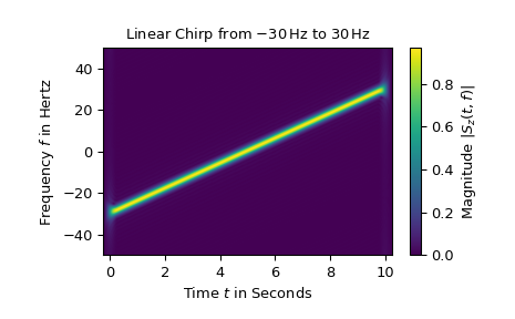
請注意,使用負頻率僅對複數值訊號才有意義。此外,複數指數函數的幅度為 1,而實數值餘弦函數的幅度僅為 1/2。