cumulative_simpson#
- scipy.integrate.cumulative_simpson(y, *, x=None, dx=1.0, axis=-1, initial=None)[source]#
使用複合辛普森 1/3 規則累積積分 y(x)。每個點的樣本積分是通過假設每個點與兩個相鄰點之間的二次關係來計算的。
- 參數:
- y類陣列
要積分的值。沿 axis 軸至少需要一個點。如果沿 axis 軸提供的點少於或等於兩個,則辛普森積分不可行,結果將使用
cumulative_trapezoid計算。- x類陣列,選用
要沿其積分的座標。必須與 y 具有相同的形狀,或者必須是 1D 且沿 axis 軸與 y 具有相同的長度。x 也必須沿 axis 軸嚴格遞增。如果 x 為 None (預設值),則使用 y 中連續元素之間的間距 dx 執行積分。
- dx純量或類陣列,選用
y 元素之間的間距。僅在 x 為 None 時使用。可以是浮點數,也可以是與 y 具有相同形狀的陣列,但在 axis 軸上的長度為 1。預設值為 1.0。
- axis整數,選用
指定要沿其積分的軸。預設值為 -1 (最後一個軸)。
- initial純量或類陣列,選用
如果給定,則將此值插入到返回結果的開頭,並將其添加到結果的其餘部分。預設值為 None,這表示不返回
x[0]的值,並且 res 沿積分軸比 y 少一個元素。可以是浮點數,也可以是與 y 具有相同形狀的陣列,但在 axis 軸上的長度為 1。
- 返回:
- resndarray
沿 axis 軸對 y 進行累積積分的結果。如果 initial 為 None,則形狀使得積分軸的值比 y 少一個。如果給定了 initial,則形狀與 y 的形狀相同。
另請參閱
numpy.cumsumcumulative_trapezoid使用複合梯形規則進行累積積分
simpson使用複合辛普森規則對採樣數據進行積分
註解
在版本 1.12.0 中新增。
複合辛普森 1/3 法可用於近似採樣輸入函數 \(y(x)\) [1] 的定積分。該方法假設在包含任何三個連續採樣點的區間上存在二次關係。
考慮三個連續點:\((x_1, y_1), (x_2, y_2), (x_3, y_3)\)。
假設這三個點之間存在二次關係,則 \(x_1\) 和 \(x_2\) 之間子區間的積分由 [2] 的公式 (8) 給出
\[\begin{split}\int_{x_1}^{x_2} y(x) dx\ &= \frac{x_2-x_1}{6}\left[\ \left\{3-\frac{x_2-x_1}{x_3-x_1}\right\} y_1 + \ \left\{3 + \frac{(x_2-x_1)^2}{(x_3-x_2)(x_3-x_1)} + \ \frac{x_2-x_1}{x_3-x_1}\right\} y_2\\ - \frac{(x_2-x_1)^2}{(x_3-x_2)(x_3-x_1)} y_3\right]\end{split}\]介於 \(x_2\) 和 \(x_3\) 之間的積分是通過交換 \(x_1\) 和 \(x_3\) 的位置給出的。積分是針對每個子區間單獨估算的,然後累積求和以獲得最終結果。
對於等間隔的樣本,如果函數是三次或更低階的多項式 [1] 且子區間數為偶數,則結果是精確的。否則,積分對於二次或更低階的多項式是精確的。
參考文獻
[2]Cartwright, Kenneth V. Simpson’s Rule Cumulative Integration with MS Excel and Irregularly-spaced Data. Journal of Mathematical Sciences and Mathematics Education. 12 (2): 1-9
範例
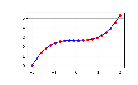
>>> from scipy import integrate
>>> import numpy as np
>>> import matplotlib.pyplot as plt
>>> x = np.linspace(-2, 2, num=20)
>>> y = x**2
>>> y_int = integrate.cumulative_simpson(y, x=x, initial=0)
>>> fig, ax = plt.subplots()
>>> ax.plot(x, y_int, 'ro', x, x**3/3 - (x[0])**3/3, 'b-')
>>> ax.grid()
>>> plt.show()
cumulative_simpson的輸出與迭代調用simpson並逐步提高積分上限的輸出相似,但不完全相同。>>> def cumulative_simpson_reference(y, x): ... return np.asarray([integrate.simpson(y[:i], x=x[:i]) ... for i in range(2, len(y) + 1)]) >>> >>> rng = np.random.default_rng() >>> x, y = rng.random(size=(2, 10)) >>> x.sort() >>> >>> res = integrate.cumulative_simpson(y, x=x) >>> ref = cumulative_simpson_reference(y, x) >>> equal = np.abs(res - ref) < 1e-15 >>> equal # not equal when `simpson` has even number of subintervals array([False, True, False, True, False, True, False, True, True])
這是預期的:因為
cumulative_simpson比simpson可以訪問更多資訊,因此它通常可以產生更準確的子區間基礎積分估計。