fht#
- scipy.fft.fht(a, dln, mu, offset=0.0, bias=0.0)[原始碼]#
計算快速漢克爾轉換。
使用 FFTLog 演算法 [1], [2],計算對數間隔週期序列的離散漢克爾轉換。
- 參數:
- aarray_like (…, n)
實數週期輸入陣列,均勻對數間隔。對於多維輸入,轉換將在最後一個軸上執行。
- dlnfloat
輸入陣列的均勻對數間隔。
- mufloat
漢克爾轉換的階數,任何正或負實數。
- offsetfloat, optional
輸出陣列均勻對數間隔的偏移量。
- biasfloat, optional
冪律偏差的指數,任何正或負實數。
- 返回:
- Aarray_like (…, n)
轉換後的輸出陣列,它是實數、週期性、均勻對數間隔的,並且形狀與輸入陣列相同。
註釋
此函數計算漢克爾轉換的離散版本
\[A(k) = \int_{0}^{\infty} \! a(r) \, J_\mu(kr) \, k \, dr \;,\]其中 \(J_\mu\) 是 \(\mu\) 階的貝索函數。索引 \(\mu\) 可以是任何實數,正數或負數。請注意,數值漢克爾轉換使用 \(k \, dr\) 的被積函數,而數學漢克爾轉換通常使用 \(r \, dr\) 定義。
輸入陣列 a 是一個長度為 \(n\) 的週期序列,均勻對數間隔,間隔為 dln,
\[a_j = a(r_j) \;, \quad r_j = r_c \exp[(j-j_c) \, \mathtt{dln}]\]以點 \(r_c\) 為中心。 請注意,如果 \(n\) 是偶數,則中心索引 \(j_c = (n-1)/2\) 是半整數,因此 \(r_c\) 落在兩個輸入元素之間。 同樣地,輸出陣列 A 是一個長度為 \(n\) 的週期序列,也以間隔 dln 均勻對數間隔
\[A_j = A(k_j) \;, \quad k_j = k_c \exp[(j-j_c) \, \mathtt{dln}]\]以點 \(k_c\) 為中心。
週期區間的中心點 \(r_c\) 和 \(k_c\) 可以任意選擇,但通常會選擇乘積 \(k_c r_c = k_j r_{n-1-j} = k_{n-1-j} r_j\) 為單位。 這可以使用 offset 參數更改,該參數控制輸出陣列的對數偏移量 \(\log(k_c) = \mathtt{offset} - \log(r_c)\)。 為 offset 選擇最佳值可以減少離散漢克爾轉換的振盪。
如果 bias 參數是非零值,則此函數計算有偏差的漢克爾轉換的離散版本
\[A(k) = \int_{0}^{\infty} \! a_q(r) \, (kr)^q \, J_\mu(kr) \, k \, dr\]其中 \(q\) 是 bias 的值,並且將冪律偏差 \(a_q(r) = a(r) \, (kr)^{-q}\) 應用於輸入序列。 如果存在一個值 \(q\) 使得 \(a_q(r)\) 接近週期序列,則偏差轉換可以幫助近似 \(a(r)\) 的連續轉換,在這種情況下,結果 \(A(k)\) 將接近連續轉換。
參考文獻
[1]Talman J. D., 1978, J. Comp. Phys., 29, 35
範例
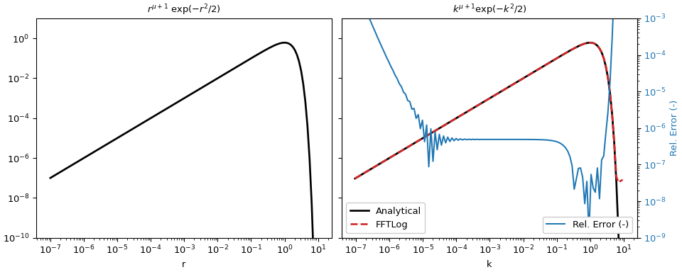
此範例是 [2] 中提供的
fftlogtest.f的改編版本。 它評估積分\[\int^\infty_0 r^{\mu+1} \exp(-r^2/2) J_\mu(kr) k dr = k^{\mu+1} \exp(-k^2/2) .\]>>> import numpy as np >>> from scipy import fft >>> import matplotlib.pyplot as plt
轉換的參數。
>>> mu = 0.0                     # Order mu of Bessel function
>>> r = np.logspace(-7, 1, 128)  # Input evaluation points
>>> dln = np.log(r[1]/r[0])      # Step size
>>> offset = fft.fhtoffset(dln, initial=-6*np.log(10), mu=mu)
>>> k = np.exp(offset)/r[::-1]   # Output evaluation points
定義解析函數。
>>> def f(x, mu):
...     """Analytical function: x^(mu+1) exp(-x^2/2)."""
...     return x**(mu + 1)*np.exp(-x**2/2)
在
r處評估函數,並使用 FFTLog 計算k處的對應值。>>> a_r = f(r, mu) >>> fht = fft.fht(a_r, dln, mu=mu, offset=offset)
在此範例中,我們實際上可以計算解析響應(在本例中與輸入函數相同)以進行比較並計算相對誤差。
>>> a_k = f(k, mu)
>>> rel_err = abs((fht-a_k)/a_k)
繪製結果。
>>> figargs = {'sharex': True, 'sharey': True, 'constrained_layout': True}
>>> fig, (ax1, ax2) = plt.subplots(1, 2, figsize=(10, 4), **figargs)
>>> ax1.set_title(r'$r^{\mu+1}\ \exp(-r^2/2)$')
>>> ax1.loglog(r, a_r, 'k', lw=2)
>>> ax1.set_xlabel('r')
>>> ax2.set_title(r'$k^{\mu+1} \exp(-k^2/2)$')
>>> ax2.loglog(k, a_k, 'k', lw=2, label='Analytical')
>>> ax2.loglog(k, fht, 'C3--', lw=2, label='FFTLog')
>>> ax2.set_xlabel('k')
>>> ax2.legend(loc=3, framealpha=1)
>>> ax2.set_ylim([1e-10, 1e1])
>>> ax2b = ax2.twinx()
>>> ax2b.loglog(k, rel_err, 'C0', label='Rel. Error (-)')
>>> ax2b.set_ylabel('Rel. Error (-)', color='C0')
>>> ax2b.tick_params(axis='y', labelcolor='C0')
>>> ax2b.legend(loc=4, framealpha=1)
>>> ax2b.set_ylim([1e-9, 1e-3])
>>> plt.show()