外插提示與技巧#
外插的處理方式—在內插資料域之外的查詢點上評估內插器—在 scipy.interpolate 中的不同常式之間並不完全一致。不同的內插器使用不同的關鍵字引數集來控制資料域之外的行為:有些使用 extrapolate=True/False/None,有些允許 fill_value 關鍵字。請參閱 API 文件以了解每個特定內插常式的詳細資訊。
根據特定問題,可用的關鍵字可能足夠或不足夠。對於非線性內插器的外插,需要特別注意。通常,隨著與資料域距離的增加,外插結果變得越來越沒有意義。這當然是可以預期的:內插器只知道資料域內的資料。
當預設的外插結果不足時,使用者需要自行實作所需的外插模式。
在本教學中,我們考慮了幾個範例,在這些範例中,我們示範了可用關鍵字的使用以及所需外插模式的手動實作。這些範例可能適用於您的特定問題,也可能不適用;它們不一定是最佳實務;並且它們經過刻意簡化,僅保留了示範主要概念所需的基本要素,希望它們能為您處理特定問題提供靈感。
interp1d : 複製 numpy.interp 的左右填充值#
重點摘要:使用 fill_value=(left, right)
numpy.interp 使用常數外插,並預設為擴展內插區間中 y 陣列的第一個和最後一個值:np.interp(xnew, x, y) 的輸出對於 xnew < x[0] 是 y[0],對於 xnew > x[-1] 是 y[-1]。
預設情況下,interp1d 拒絕外插,並且當在內插範圍之外的資料點上評估時,會引發 ValueError。這可以通過 bounds_error=False 引數關閉:然後 interp1d 使用 fill_value 設定超出範圍的值,預設情況下 fill_value 為 nan。
為了模擬 numpy.interp 與 interp1d 的行為,您可以使用它支援 2 元組作為 fill_value 的事實。然後,元組元素用於填充 xnew < min(x) 和 x > max(x) 的值。對於多維 y,這些元素必須具有與 y 相同的形狀,或者可以廣播到它。
為了說明
import numpy as np
import matplotlib.pyplot as plt
from scipy.interpolate import interp1d

x = np.linspace(0, 1.5*np.pi, 11)
y = np.column_stack((np.cos(x), np.sin(x)))   # y.shape is (11, 2)

func = interp1d(x, y,
                axis=0,  # interpolate along columns
                bounds_error=False,
                kind='linear',
                fill_value=(y[0], y[-1]))
xnew = np.linspace(-np.pi, 2.5*np.pi, 51)
ynew = func(xnew)

fix, (ax1, ax2) = plt.subplots(1, 2, figsize=(8, 4))
ax1.plot(xnew, ynew[:, 0])
ax1.plot(x, y[:, 0], 'o')

ax2.plot(xnew, ynew[:, 1])
ax2.plot(x, y[:, 1], 'o')
plt.tight_layout()
CubicSpline 擴展邊界條件#
CubicSpline 需要兩個額外的邊界條件,這些條件由 bc_type 參數控制。此參數可以列出邊緣處導數的明確值,或使用有用的別名。例如,bc_type="clamped" 將一階導數設定為零,bc_type="natural" 將二階導數設定為零(另外兩個公認的字串值是 “periodic” 和 “not-a-knot”)
雖然外插是由邊界條件控制的,但這種關係不是很直觀。例如,人們可能會預期對於 bc_type="natural",外插是線性的。這種期望太強了:每個邊界條件僅在單個點(僅在邊界)設定導數。外插是從第一個和最後一個多項式片段完成的,對於自然樣條,這是一個在給定點處具有零二階導數的三次多項式。
理解為什麼這種期望太強的另一種方法是考慮只有三個資料點的資料集,其中樣條有兩個多項式片段。為了線性外插,這種期望意味著這兩個片段都是線性的。但是,兩個線性片段無法在中間點以連續的二階導數匹配!(除非當然,所有三個資料點實際上都位於單一直線上)。
為了說明這種行為,我們考慮一個合成資料集並比較幾個邊界條件
import numpy as np
import matplotlib.pyplot as plt
from scipy.interpolate import CubicSpline

xs = [1, 2, 3, 4, 5, 6, 7, 8]
ys = [4.5, 3.6, 1.6, 0.0, -3.3, -3.1, -1.8, -1.7]

notaknot = CubicSpline(xs, ys, bc_type='not-a-knot')
natural = CubicSpline(xs, ys, bc_type='natural')
clamped = CubicSpline(xs, ys, bc_type='clamped')
xnew = np.linspace(min(xs) - 4, max(xs) + 4, 101)

splines = [notaknot, natural, clamped]
titles = ['not-a-knot', 'natural', 'clamped']

fig, axs = plt.subplots(3, 3, figsize=(12, 12))
for i in [0, 1, 2]:
    for j, spline, title in zip(range(3), splines, titles):
        axs[i, j].plot(xs, spline(xs, nu=i),'o')
        axs[i, j].plot(xnew, spline(xnew, nu=i),'-')
        axs[i, j].set_title(f'{title}, deriv={i}')

plt.tight_layout()
plt.show()
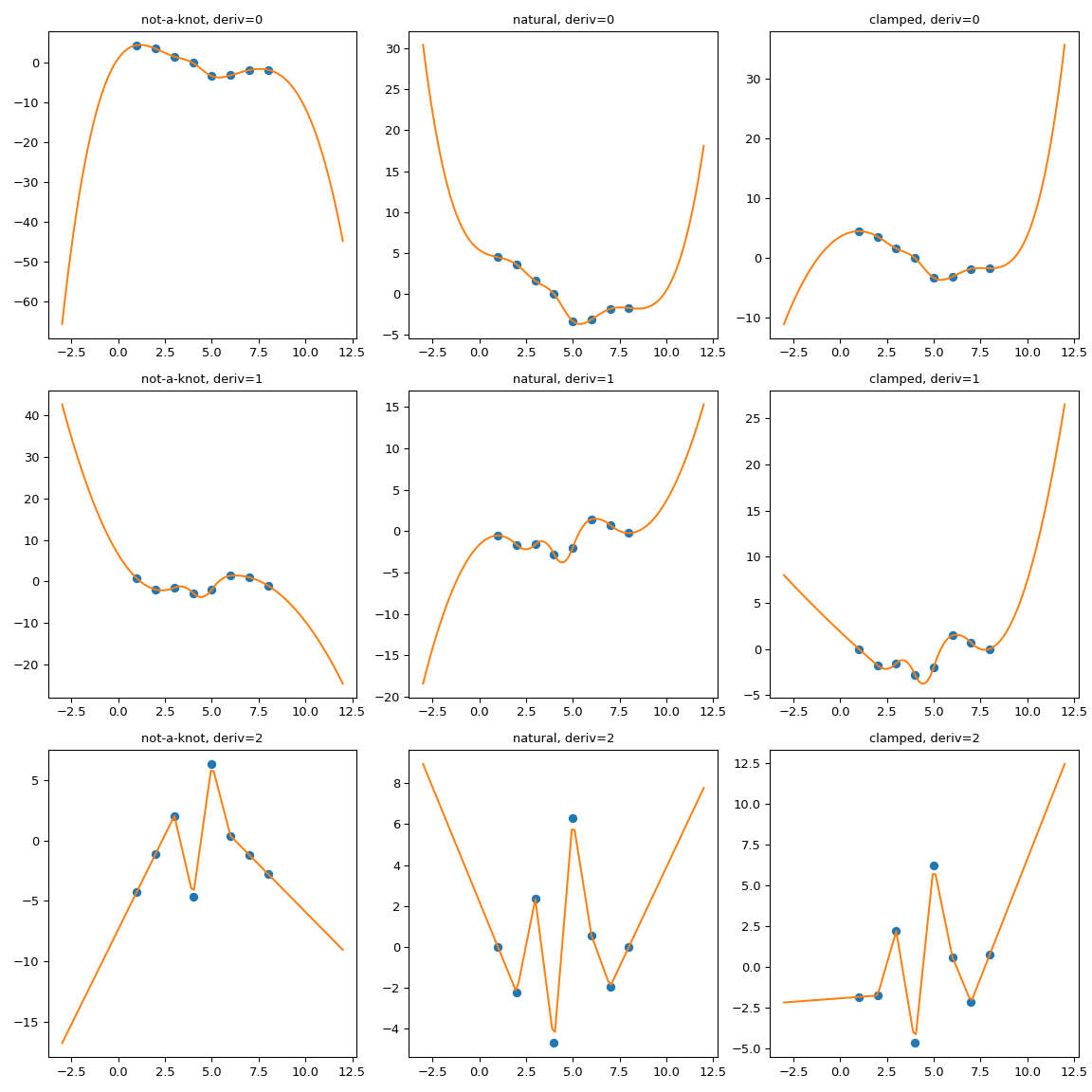
可以清楚地看到,自然樣條在邊界處確實具有零二階導數,但外插是非線性的。bc_type="clamped" 顯示出類似的行為:一階導數僅在邊界處完全等於零。在所有情況下,外插都是通過擴展樣條的第一個和最後一個多項式片段來完成的,無論它們碰巧是什麼。
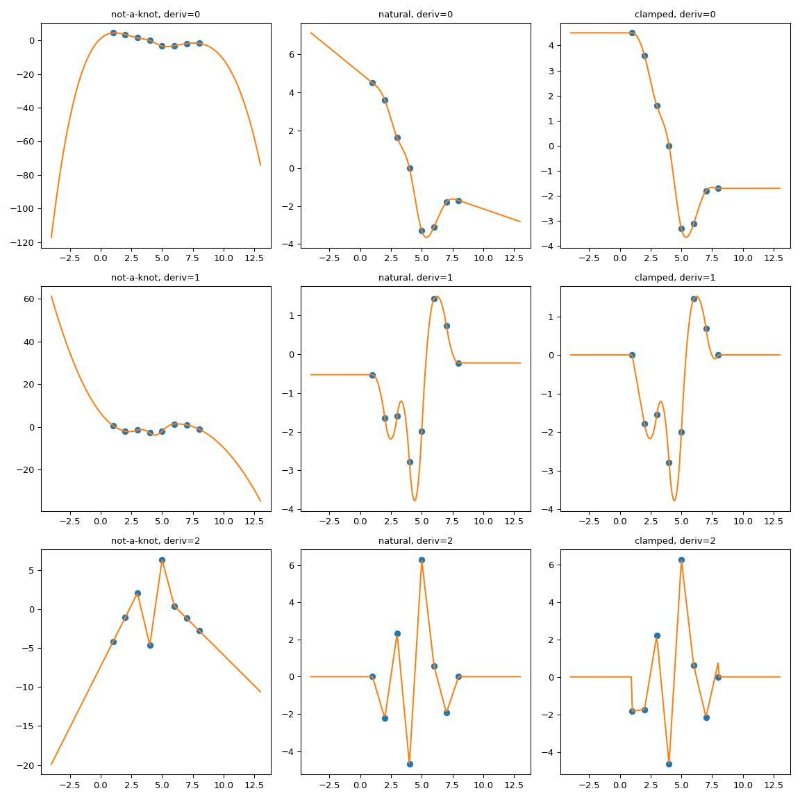
強制外插的一種可能方法是擴展內插域,以添加具有所需屬性的第一個和最後一個多項式片段。
在這裡,我們使用 CubicSpline 超類別 PPoly 的 extend 方法,以添加兩個額外的斷點,並確保額外的多項式片段保持導數的值。然後,外插使用這兩個額外的區間繼續進行。
import numpy as np
import matplotlib.pyplot as plt
from scipy.interpolate import CubicSpline

def add_boundary_knots(spline):
    """
    Add knots infinitesimally to the left and right.

    Additional intervals are added to have zero 2nd and 3rd derivatives,
    and to maintain the first derivative from whatever boundary condition
    was selected. The spline is modified in place.
    """
    # determine the slope at the left edge
    leftx = spline.x[0]
    lefty = spline(leftx)
    leftslope = spline(leftx, nu=1)

    # add a new breakpoint just to the left and use the
    # known slope to construct the PPoly coefficients.
    leftxnext = np.nextafter(leftx, leftx - 1)
    leftynext = lefty + leftslope*(leftxnext - leftx)
    leftcoeffs = np.array([0, 0, leftslope, leftynext])
    spline.extend(leftcoeffs[..., None], np.r_[leftxnext])

    # repeat with additional knots to the right
    rightx = spline.x[-1]
    righty = spline(rightx)
    rightslope = spline(rightx,nu=1)
    rightxnext = np.nextafter(rightx, rightx + 1)
    rightynext = righty + rightslope * (rightxnext - rightx)
    rightcoeffs = np.array([0, 0, rightslope, rightynext])
    spline.extend(rightcoeffs[..., None], np.r_[rightxnext])

xs = [1, 2, 3, 4, 5, 6, 7, 8]
ys = [4.5, 3.6, 1.6, 0.0, -3.3, -3.1, -1.8, -1.7]

notaknot = CubicSpline(xs,ys, bc_type='not-a-knot')
# not-a-knot does not require additional intervals

natural = CubicSpline(xs,ys, bc_type='natural')
# extend the natural natural spline with linear extrapolating knots
add_boundary_knots(natural)

clamped = CubicSpline(xs,ys, bc_type='clamped')
# extend the clamped spline with constant extrapolating knots
add_boundary_knots(clamped)

xnew = np.linspace(min(xs) - 5, max(xs) + 5, 201)

fig, axs = plt.subplots(3, 3,figsize=(12,12))

splines = [notaknot, natural, clamped]
titles = ['not-a-knot', 'natural', 'clamped']

for i in [0, 1, 2]:
    for j, spline, title in zip(range(3), splines, titles):
        axs[i, j].plot(xs, spline(xs, nu=i),'o')
        axs[i, j].plot(xnew, spline(xnew, nu=i),'-')
        axs[i, j].set_title(f'{title}, deriv={i}')

plt.tight_layout()
plt.show()
手動實作漸近線#
先前擴展內插域的技巧依賴於 CubicSpline.extend 方法。一種稍微更通用的替代方法是實作一個包裝函式,該包裝函式顯式處理超出範圍的行為。讓我們考慮一個範例。
設定#
假設我們想在給定的 \(a\) 值下求解方程式
(這些方程式出現的一個應用是在求解量子粒子的能級)。為了簡化起見,我們僅考慮 \(x\in (0, \pi/2)\)。
一次求解此方程式很簡單
import numpy as np
import matplotlib.pyplot as plt
from scipy.optimize import brentq

def f(x, a):
    return a*x - 1/np.tan(x)

a = 3
x0 = brentq(f, 1e-16, np.pi/2, args=(a,))   # here we shift the left edge
                                            # by a machine epsilon to avoid
                                            # a division by zero at x=0
xx = np.linspace(0.2, np.pi/2, 101)
plt.plot(xx, a*xx, '--')
plt.plot(xx, 1/np.tan(xx), '--')
plt.plot(x0, a*x0, 'o', ms=12)
plt.text(0.1, 0.9, fr'$x_0 = {x0:.3f}$',
               transform=plt.gca().transAxes, fontsize=16)
plt.show()
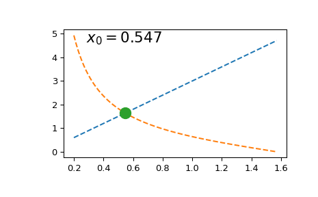
但是,如果我們需要多次求解它(例如,由於 tan 函數的週期性而尋找一系列根),則重複呼叫 scipy.optimize.brentq 會變得非常昂貴。
為了規避這個困難,我們將 \(y = ax - 1/\tan{x}\) 製成表格,並在表格化的網格上內插它。實際上,我們將使用反向內插:我們內插 \(x\) 相對於 \(у\) 的值。這樣,求解原始方程式就簡化為在零 \(y\) 引數下評估內插函數。
為了提高內插準確性,我們將使用表格化函數導數的知識。我們將使用 BPoly.from_derivatives 來建構三次內插器(或者,我們可以使用 CubicHermiteSpline)
import numpy as np
import matplotlib.pyplot as plt
from scipy.interpolate import BPoly

def f(x, a):
    return a*x - 1/np.tan(x)

xleft, xright = 0.2, np.pi/2
x = np.linspace(xleft, xright, 11)

fig, ax = plt.subplots(1, 2, figsize=(12, 4))

for j, a in enumerate([3, 93]):
    y = f(x, a)
    dydx = a + 1./np.sin(x)**2    # d(ax - 1/tan(x)) / dx
    dxdy = 1 / dydx               # dx/dy = 1 / (dy/dx)

    xdx = np.c_[x, dxdy]
    spl = BPoly.from_derivatives(y, xdx)   # inverse interpolation

    yy = np.linspace(f(xleft, a), f(xright, a), 51)
    ax[j].plot(yy, spl(yy), '--')
    ax[j].plot(y, x, 'o')
    ax[j].set_xlabel(r'$y$')
    ax[j].set_ylabel(r'$x$')
    ax[j].set_title(rf'$a = {a}$')

    ax[j].plot(0, spl(0), 'o', ms=12)
    ax[j].text(0.1, 0.85, fr'$x_0 = {spl(0):.3f}$',
               transform=ax[j].transAxes, fontsize=18)
    ax[j].grid(True)
plt.tight_layout()
plt.show()
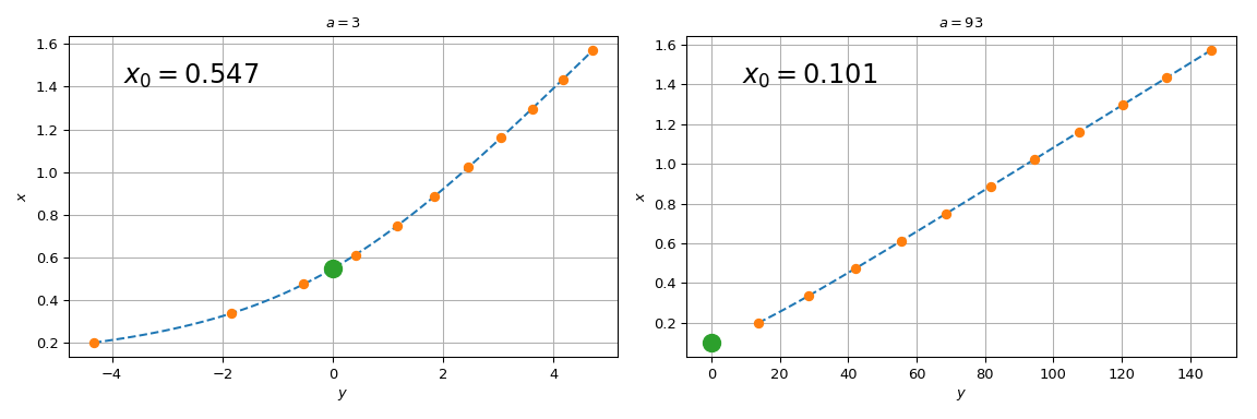
請注意,對於 \(a=3\),spl(0) 與上面的 brentq 呼叫一致,而對於 \(a = 93\),差異很大。對於較大的 \(a\),程序開始失敗的原因是直線 \(y = ax\) 趨向於垂直軸,而原始方程式的根趨向於 \(x=0\)。由於我們在有限網格上對原始函數進行了表格化,因此對於太大的 \(a\) 值,spl(0) 涉及外插。依賴外插容易失去準確性,最好避免。
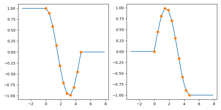
使用已知的漸近線#
查看原始方程式,我們注意到對於 \(x\to 0\),\(\tan(x) = x + O(x^3)\),原始方程式變為
因此對於 \(a \gg 1\),\(x_0 \approx 1/\sqrt{a}\)。
我們將使用它來建立一個類別,該類別從內插切換為對超出範圍的資料使用此已知的漸近行為。一個最基本的實作可能如下所示
class RootWithAsymptotics:
   def __init__(self, a):

       # construct the interpolant
       xleft, xright = 0.2, np.pi/2
       x = np.linspace(xleft, xright, 11)

       y = f(x, a)
       dydx = a + 1./np.sin(x)**2    # d(ax - 1/tan(x)) / dx
       dxdy = 1 / dydx               # dx/dy = 1 / (dy/dx)

       # inverse interpolation
       self.spl = BPoly.from_derivatives(y, np.c_[x, dxdy])
       self.a = a

   def root(self):
       out = self.spl(0)
       asympt = 1./np.sqrt(self.a)
       return np.where(spl.x.min() < asympt, out, asympt)
然後
>>> r = RootWithAsymptotics(93)
>>> r.root()
array(0.10369517)
這與外插結果不同,但與 brentq 呼叫一致。
請注意,此實作是故意簡化的。從 API 的角度來看,您可能希望改為實作 __call__ 方法,以便可以使用 x 對 y 的完整依賴關係。從數值的角度來看,需要做更多工作以確保內插和漸近線之間的切換發生在足夠深入漸近區域的位置,以便產生的函數在切換點處足夠平滑。
同樣在本範例中,我們人為地將問題限制為僅考慮 tan 函數的單個週期區間,並且僅處理 \(a > 0\)。對於 \(a\) 的負值,我們將需要實作另一個漸近線,即對於 \(x\to \pi\)。
但是基本概念是相同的。
D > 1 中的外插#
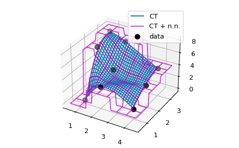
在包裝函式類別或函數中手動實作外插的基本概念可以很容易地推廣到更高的維度。作為一個範例,我們考慮使用 CloughTocher2DInterpolator 進行二維資料的 C1 平滑內插問題。預設情況下,它使用 nan 填充超出範圍的值,我們希望改為對每個查詢點使用其最近鄰居的值。
由於 CloughTocher2DInterpolator 接受二維資料或資料點的 Delaunay 三角剖分,因此尋找查詢點最近鄰居的有效方法是建構三角剖分(使用 scipy.spatial 工具)並使用它在資料的凸包上尋找最近鄰居。
我們將改為使用更簡單、更原始的方法,並依賴於使用 NumPy 廣播對整個資料集進行迴圈。
import numpy as np
import matplotlib.pyplot as plt
from scipy.interpolate import CloughTocher2DInterpolator as CT

def my_CT(xy, z):
    """CT interpolator + nearest-neighbor extrapolation.

    Parameters
    ----------
    xy : ndarray, shape (npoints, ndim)
        Coordinates of data points
    z : ndarray, shape (npoints)
        Values at data points

    Returns
    -------
    func : callable
        A callable object which mirrors the CT behavior,
        with an additional neareast-neighbor extrapolation
        outside of the data range.
    """
    x = xy[:, 0]
    y = xy[:, 1]
    f = CT(xy, z)

    # this inner function will be returned to a user
    def new_f(xx, yy):
        # evaluate the CT interpolator. Out-of-bounds values are nan.
        zz = f(xx, yy)
        nans = np.isnan(zz)

        if nans.any():
            # for each nan point, find its nearest neighbor
            inds = np.argmin(
                (x[:, None] - xx[nans])**2 +
                (y[:, None] - yy[nans])**2
                , axis=0)
            # ... and use its value
            zz[nans] = z[inds]
        return zz

    return new_f

# Now illustrate the difference between the original ``CT`` interpolant
# and ``my_CT`` on a small example:

x = np.array([1, 1, 1, 2, 2, 2, 4, 4, 4])
y = np.array([1, 2, 3, 1, 2, 3, 1, 2, 3])
z = np.array([0, 7, 8, 3, 4, 7, 1, 3, 4])

xy = np.c_[x, y]
lut = CT(xy, z)
lut2 = my_CT(xy, z)

X = np.linspace(min(x) - 0.5, max(x) + 0.5, 71)
Y = np.linspace(min(y) - 0.5, max(y) + 0.5, 71)
X, Y = np.meshgrid(X, Y)

fig = plt.figure()
ax = fig.add_subplot(projection='3d')

ax.plot_wireframe(X, Y, lut(X, Y), label='CT')
ax.plot_wireframe(X, Y, lut2(X, Y), color='m',
                  cstride=10, rstride=10, alpha=0.7, label='CT + n.n.')

ax.scatter(x, y, z,  'o', color='k', s=48, label='data')
ax.legend()
plt.tight_layout()