最佳化 (scipy.optimize)

scipy.optimize 套件提供數種常用的最佳化演算法。詳細列表請見：scipy.optimize (也可以透過 help(scipy.optimize) 找到)。

多變數純量函數的局部最佳化 (minimize)

minimize 函數為 scipy.optimize 中多變數純量函數的非約束和約束最佳化演算法提供通用介面。為了示範最佳化函數，請考慮最小化 \(N\) 個變數的 Rosenbrock 函數問題

\[f\left(\mathbf{x}\right)=\sum_{i=1}^{N-1}100\left(x_{i+1}-x_{i}^{2}\right)^{2}+\left(1-x_{i}\right)^{2}.\]

此函數的最小值為 0，當 \(x_{i}=1.\) 時達到。

請注意，Rosenbrock 函數及其導數包含在 scipy.optimize 中。以下章節中顯示的實作範例說明如何定義目標函數及其 Jacobian 函數和 Hessian 函數。scipy.optimize 中的目標函數預期將 NumPy 陣列作為其要最佳化的第一個參數，並且必須傳回浮點數值。確切的呼叫簽名必須是 f(x, *args)，其中 x 代表 NumPy 陣列，而 args 是一個提供給目標函數的額外引數元組。

非約束最佳化

Nelder-Mead 單純形演算法 (method='Nelder-Mead')

在以下範例中，minimize 常式與 Nelder-Mead 單純形演算法 (透過 method 參數選取) 一起使用

>>> import numpy as np
>>> from scipy.optimize import minimize

>>> def rosen(x):
...     """The Rosenbrock function"""
...     return sum(100.0*(x[1:]-x[:-1]**2.0)**2.0 + (1-x[:-1])**2.0)

>>> x0 = np.array([1.3, 0.7, 0.8, 1.9, 1.2])
>>> res = minimize(rosen, x0, method='nelder-mead',
...                options={'xatol': 1e-8, 'disp': True})
Optimization terminated successfully.
         Current function value: 0.000000
         Iterations: 339
         Function evaluations: 571

>>> print(res.x)
[1. 1. 1. 1. 1.]

單純形演算法可能是最小化行為良好的函數的最簡單方法。它只需要函數評估，並且是簡單最小化問題的理想選擇。但是，由於它不使用任何梯度評估，因此可能需要更長的時間才能找到最小值。

另一個只需要函數呼叫即可找到最小值的最佳化演算法是 Powell 方法，可以透過在 minimize 中設定 method='powell' 來使用。

為了示範如何向目標函數提供額外引數，讓我們最小化具有額外縮放因子 a 和偏移量 b 的 Rosenbrock 函數

\[f\left(\mathbf{x}, a, b\right)=\sum_{i=1}^{N-1}a\left(x_{i+1}-x_{i}^{2}\right)^{2}+\left(1-x_{i}\right)^{2} + b.\]

再次使用 minimize 常式，可以透過以下程式碼區塊針對範例參數 a=0.5 和 b=1 求解。

>>> def rosen_with_args(x, a, b):
...     """The Rosenbrock function with additional arguments"""
...     return sum(a*(x[1:]-x[:-1]**2.0)**2.0 + (1-x[:-1])**2.0) + b

>>> x0 = np.array([1.3, 0.7, 0.8, 1.9, 1.2])
>>> res = minimize(rosen_with_args, x0, method='nelder-mead',
...                args=(0.5, 1.), options={'xatol': 1e-8, 'disp': True})
Optimization terminated successfully.
         Current function value: 1.000000
         Iterations: 319 # may vary
         Function evaluations: 525 # may vary

>>> print(res.x)
[1.         1.         1.         1.         0.99999999]

作為使用 minimize 的 args 參數的替代方案，只需將目標函數包裝在一個僅接受 x 的新函數中即可。當需要將額外參數作為關鍵字引數傳遞給目標函數時，此方法也很有用。

>>> def rosen_with_args(x, a, *, b):  # b is a keyword-only argument
...     return sum(a*(x[1:]-x[:-1]**2.0)**2.0 + (1-x[:-1])**2.0) + b
>>> def wrapped_rosen_without_args(x):
...     return rosen_with_args(x, 0.5, b=1.)  # pass in `a` and `b`
>>> x0 = np.array([1.3, 0.7, 0.8, 1.9, 1.2])
>>> res = minimize(wrapped_rosen_without_args, x0, method='nelder-mead',
...                options={'xatol': 1e-8,})
>>> print(res.x)
[1.         1.         1.         1.         0.99999999]

另一種替代方案是使用 functools.partial。

>>> from functools import partial
>>> partial_rosen = partial(rosen_with_args, a=0.5, b=1.)
>>> res = minimize(partial_rosen, x0, method='nelder-mead',
...                options={'xatol': 1e-8,})
>>> print(res.x)
[1.         1.         1.         1.         0.99999999]

Broyden-Fletcher-Goldfarb-Shanno 演算法 (method='BFGS')

為了更快地收斂到解，此常式使用目標函數的梯度。如果使用者未提供梯度，則會使用一階差分來估計梯度。即使必須估計梯度，Broyden-Fletcher-Goldfarb-Shanno (BFGS) 方法通常也比單純形演算法需要更少的函數呼叫。

為了示範此演算法，再次使用 Rosenbrock 函數。Rosenbrock 函數的梯度是向量

\begin{eqnarray*} \frac{\partial f}{\partial x_{j}} & = & \sum_{i=1}^{N}200\left(x_{i}-x_{i-1}^{2}\right)\left(\delta_{i,j}-2x_{i-1}\delta_{i-1,j}\right)-2\left(1-x_{i-1}\right)\delta_{i-1,j}.\\ & = & 200\left(x_{j}-x_{j-1}^{2}\right)-400x_{j}\left(x_{j+1}-x_{j}^{2}\right)-2\left(1-x_{j}\right).\end{eqnarray*}

此表達式對內部導數有效。特殊情況是

\begin{eqnarray*} \frac{\partial f}{\partial x_{0}} & = & -400x_{0}\left(x_{1}-x_{0}^{2}\right)-2\left(1-x_{0}\right),\\ \frac{\partial f}{\partial x_{N-1}} & = & 200\left(x_{N-1}-x_{N-2}^{2}\right).\end{eqnarray*}

計算此梯度的 Python 函數由程式碼片段建構

>>> def rosen_der(x):
...     xm = x[1:-1]
...     xm_m1 = x[:-2]
...     xm_p1 = x[2:]
...     der = np.zeros_like(x)
...     der[1:-1] = 200*(xm-xm_m1**2) - 400*(xm_p1 - xm**2)*xm - 2*(1-xm)
...     der[0] = -400*x[0]*(x[1]-x[0]**2) - 2*(1-x[0])
...     der[-1] = 200*(x[-1]-x[-2]**2)
...     return der

此梯度資訊在 minimize 函數中透過 jac 參數指定，如下所示。

>>> res = minimize(rosen, x0, method='BFGS', jac=rosen_der,
...                options={'disp': True})
Optimization terminated successfully.
         Current function value: 0.000000
         Iterations: 25                     # may vary
         Function evaluations: 30
         Gradient evaluations: 30
>>> res.x
array([1., 1., 1., 1., 1.])

避免冗餘計算

目標函數及其梯度通常會共用部分計算。例如，考慮以下問題。

>>> def f(x):
...    return -expensive(x[0])**2
>>>
>>> def df(x):
...     return -2 * expensive(x[0]) * dexpensive(x[0])
>>>
>>> def expensive(x):
...     # this function is computationally expensive!
...     expensive.count += 1  # let's keep track of how many times it runs
...     return np.sin(x)
>>> expensive.count = 0
>>>
>>> def dexpensive(x):
...     return np.cos(x)
>>>
>>> res = minimize(f, 0.5, jac=df)
>>> res.fun
-0.9999999999999174
>>> res.nfev, res.njev
6, 6
>>> expensive.count
12

在這裡，expensive 被呼叫了 12 次：目標函數中 6 次，梯度中 6 次。減少冗餘計算的一種方法是建立一個傳回目標函數和梯度的單一函數。

>>> def f_and_df(x):
...     expensive_value = expensive(x[0])
...     return (-expensive_value**2,  # objective function
...             -2*expensive_value*dexpensive(x[0]))  # gradient
>>>
>>> expensive.count = 0  # reset the counter
>>> res = minimize(f_and_df, 0.5, jac=True)
>>> res.fun
-0.9999999999999174
>>> expensive.count
6

當我們呼叫 minimize 時，我們指定 jac==True 以指示提供的函數傳回目標函數及其梯度。雖然方便，但並非所有 scipy.optimize 函數都支援此功能，而且，它僅適用於在函數及其梯度之間共用計算，而在某些問題中，我們會想要與 Hessian (目標函數的二階導數) 和約束共用計算。更通用的方法是記憶化計算的昂貴部分。在簡單的情況下，可以使用 functools.lru_cache 包裝器來完成此操作。

>>> from functools import lru_cache
>>> expensive.count = 0  # reset the counter
>>> expensive = lru_cache(expensive)
>>> res = minimize(f, 0.5, jac=df)
>>> res.fun
-0.9999999999999174
>>> expensive.count
6

Newton-共軛梯度演算法 (method='Newton-CG')

Newton-共軛梯度演算法是一種修改後的 Newton 方法，它使用共軛梯度演算法來 (近似) 反轉局部 Hessian [NW]。Newton 方法基於將函數局部擬合為二次形式

\[f\left(\mathbf{x}\right)\approx f\left(\mathbf{x}_{0}\right)+\nabla f\left(\mathbf{x}_{0}\right)\cdot\left(\mathbf{x}-\mathbf{x}_{0}\right)+\frac{1}{2}\left(\mathbf{x}-\mathbf{x}_{0}\right)^{T}\mathbf{H}\left(\mathbf{x}_{0}\right)\left(\mathbf{x}-\mathbf{x}_{0}\right).\]

其中 \(\mathbf{H}\left(\mathbf{x}_{0}\right)\) 是二階導數 (Hessian) 的矩陣。如果 Hessian 是正定矩陣，則可以透過將二次形式的梯度設定為零來找到此函數的局部最小值，從而得到

\[\mathbf{x}_{\textrm{opt}}=\mathbf{x}_{0}-\mathbf{H}^{-1}\nabla f.\]

Hessian 的反矩陣使用共軛梯度方法進行評估。以下給出使用此方法最小化 Rosenbrock 函數的範例。為了充分利用 Newton-CG 方法，必須提供一個計算 Hessian 的函數。Hessian 矩陣本身不需要建構，只需要一個向量，該向量是 Hessian 與任意向量的乘積，即可用於最小化常式。因此，使用者可以提供一個函數來計算 Hessian 矩陣，或提供一個函數來計算 Hessian 與任意向量的乘積。

完整 Hessian 範例

Rosenbrock 函數的 Hessian 為

\begin{eqnarray*} H_{ij}=\frac{\partial^{2}f}{\partial x_{i}\partial x_{j}} & = & 200\left(\delta_{i,j}-2x_{i-1}\delta_{i-1,j}\right)-400x_{i}\left(\delta_{i+1,j}-2x_{i}\delta_{i,j}\right)-400\delta_{i,j}\left(x_{i+1}-x_{i}^{2}\right)+2\delta_{i,j},\\ & = & \left(202+1200x_{i}^{2}-400x_{i+1}\right)\delta_{i,j}-400x_{i}\delta_{i+1,j}-400x_{i-1}\delta_{i-1,j},\end{eqnarray*}

如果 \(i,j\in\left[1,N-2\right]\)，其中 \(i,j\in\left[0,N-1\right]\) 定義 \(N\times N\) 矩陣。矩陣的其他非零項為

\begin{eqnarray*} \frac{\partial^{2}f}{\partial x_{0}^{2}} & = & 1200x_{0}^{2}-400x_{1}+2,\\ \frac{\partial^{2}f}{\partial x_{0}\partial x_{1}}=\frac{\partial^{2}f}{\partial x_{1}\partial x_{0}} & = & -400x_{0},\\ \frac{\partial^{2}f}{\partial x_{N-1}\partial x_{N-2}}=\frac{\partial^{2}f}{\partial x_{N-2}\partial x_{N-1}} & = & -400x_{N-2},\\ \frac{\partial^{2}f}{\partial x_{N-1}^{2}} & = & 200.\end{eqnarray*}

例如，當 \(N=5\) 時，Hessian 為

\[\begin{split}\mathbf{H}=\begin{bmatrix} 1200x_{0}^{2}+2\mkern-2em\\&1200x_{1}^{2}+202\mkern-2em\\&&1200x_{1}^{2}+202\mkern-2em\\&&&1200x_{3}^{2}+202\mkern-1em\\&&&&200\end{bmatrix}-400\begin{bmatrix} x_1 & x_0 \\ x_0 & x_2 & x_1 \\ & x_1 & x_3 & x_2\\ & & x_2 & x_4 & x_3 \\ & & & x_3 & 0\end{bmatrix}.\end{split}\]

計算此 Hessian 的程式碼以及使用 Newton-CG 方法最小化函數的程式碼顯示在以下範例中

>>> def rosen_hess(x):
...     x = np.asarray(x)
...     H = np.diag(-400*x[:-1],1) - np.diag(400*x[:-1],-1)
...     diagonal = np.zeros_like(x)
...     diagonal[0] = 1200*x[0]**2-400*x[1]+2
...     diagonal[-1] = 200
...     diagonal[1:-1] = 202 + 1200*x[1:-1]**2 - 400*x[2:]
...     H = H + np.diag(diagonal)
...     return H

>>> res = minimize(rosen, x0, method='Newton-CG',
...                jac=rosen_der, hess=rosen_hess,
...                options={'xtol': 1e-8, 'disp': True})
Optimization terminated successfully.
         Current function value: 0.000000
         Iterations: 19                       # may vary
         Function evaluations: 22
         Gradient evaluations: 19
         Hessian evaluations: 19
>>> res.x
array([1.,  1.,  1.,  1.,  1.])

Hessian 乘積範例

對於較大的最小化問題，儲存整個 Hessian 矩陣可能會消耗大量時間和記憶體。Newton-CG 演算法只需要 Hessian 乘以任意向量的乘積。因此，使用者可以提供程式碼來計算此乘積，而不是完整的 Hessian，方法是提供一個 hess 函數，該函數將最小化向量作為第一個引數，將任意向量作為第二個引數 (以及傳遞給要最小化的函數的額外引數)。如果可能，使用具有 Hessian 乘積選項的 Newton-CG 可能是最小化函數的最快方法。

在這種情況下，Rosenbrock Hessian 與任意向量的乘積不難計算。如果 \(\mathbf{p}\) 是任意向量，則 \(\mathbf{H}\left(\mathbf{x}\right)\mathbf{p}\) 具有元素

\[\begin{split}\mathbf{H}\left(\mathbf{x}\right)\mathbf{p}=\begin{bmatrix} \left(1200x_{0}^{2}-400x_{1}+2\right)p_{0}-400x_{0}p_{1}\\ \vdots\\ -400x_{i-1}p_{i-1}+\left(202+1200x_{i}^{2}-400x_{i+1}\right)p_{i}-400x_{i}p_{i+1}\\ \vdots\\ -400x_{N-2}p_{N-2}+200p_{N-1}\end{bmatrix}.\end{split}\]

以下程式碼使用此 Hessian 乘積，透過 minimize 最小化 Rosenbrock 函數

>>> def rosen_hess_p(x, p):
...     x = np.asarray(x)
...     Hp = np.zeros_like(x)
...     Hp[0] = (1200*x[0]**2 - 400*x[1] + 2)*p[0] - 400*x[0]*p[1]
...     Hp[1:-1] = -400*x[:-2]*p[:-2]+(202+1200*x[1:-1]**2-400*x[2:])*p[1:-1] \
...                -400*x[1:-1]*p[2:]
...     Hp[-1] = -400*x[-2]*p[-2] + 200*p[-1]
...     return Hp

>>> res = minimize(rosen, x0, method='Newton-CG',
...                jac=rosen_der, hessp=rosen_hess_p,
...                options={'xtol': 1e-8, 'disp': True})
Optimization terminated successfully.
         Current function value: 0.000000
         Iterations: 20                    # may vary
         Function evaluations: 23
         Gradient evaluations: 20
         Hessian evaluations: 44
>>> res.x
array([1., 1., 1., 1., 1.])

根據 [NW] 第 170 頁，當 Hessian 由於這些情況下該方法提供的搜尋方向品質不佳而條件不良時，Newton-CG 演算法可能會效率低下。作者表示，方法 trust-ncg 更有效地處理了這種有問題的情況，接下來將對其進行說明。

信賴域 Newton-共軛梯度演算法 (method='trust-ncg')

Newton-CG 方法是一種線搜尋方法：它找到一個搜尋方向，以最小化函數的二次近似值，然後使用線搜尋演算法來找到該方向上的 (幾乎) 最佳步長。另一種方法是，首先，固定步長限制 \(\Delta\)，然後透過求解以下二次子問題，在給定的信賴域內找到最佳步長 \(\mathbf{p}\)

\begin{eqnarray*} \min_{\mathbf{p}} f\left(\mathbf{x}_{k}\right)+\nabla f\left(\mathbf{x}_{k}\right)\cdot\mathbf{p}+\frac{1}{2}\mathbf{p}^{T}\mathbf{H}\left(\mathbf{x}_{k}\right)\mathbf{p};&\\ \text{subject to: } \|\mathbf{p}\|\le \Delta.& \end{eqnarray*}

然後更新解 \(\mathbf{x}_{k+1} = \mathbf{x}_{k} + \mathbf{p}\)，並根據二次模型與實際函數的協定程度調整信賴域 \(\Delta\)。這類方法稱為信賴域方法。trust-ncg 演算法是一種信賴域方法，它使用共軛梯度演算法來求解信賴域子問題 [NW]。

完整 Hessian 範例

>>> res = minimize(rosen, x0, method='trust-ncg',
...                jac=rosen_der, hess=rosen_hess,
...                options={'gtol': 1e-8, 'disp': True})
Optimization terminated successfully.
         Current function value: 0.000000
         Iterations: 20                    # may vary
         Function evaluations: 21
         Gradient evaluations: 20
         Hessian evaluations: 19
>>> res.x
array([1., 1., 1., 1., 1.])

Hessian 乘積範例

>>> res = minimize(rosen, x0, method='trust-ncg',
...                jac=rosen_der, hessp=rosen_hess_p,
...                options={'gtol': 1e-8, 'disp': True})
Optimization terminated successfully.
         Current function value: 0.000000
         Iterations: 20                    # may vary
         Function evaluations: 21
         Gradient evaluations: 20
         Hessian evaluations: 0
>>> res.x
array([1., 1., 1., 1., 1.])

信賴域截斷廣義 Lanczos / 共軛梯度演算法 (method='trust-krylov')

與 trust-ncg 方法類似，trust-krylov 方法適用於大規模問題，因為它僅透過矩陣向量乘積將 Hessian 用作線性運算子。它比 trust-ncg 方法更準確地求解二次子問題。

\begin{eqnarray*} \min_{\mathbf{p}} f\left(\mathbf{x}_{k}\right)+\nabla f\left(\mathbf{x}_{k}\right)\cdot\mathbf{p}+\frac{1}{2}\mathbf{p}^{T}\mathbf{H}\left(\mathbf{x}_{k}\right)\mathbf{p};&\\ \text{subject to: } \|\mathbf{p}\|\le \Delta.& \end{eqnarray*}

此方法包裝了 [TRLIB] 的 [GLTR] 方法實作，該方法精確地求解了限制為截斷 Krylov 子空間的信賴域子問題。對於不定問題，通常最好使用此方法，因為與 trust-ncg 方法相比，它減少了非線性迭代的次數，但每個子問題求解需要更多矩陣向量乘積。

完整 Hessian 範例

>>> res = minimize(rosen, x0, method='trust-krylov',
...                jac=rosen_der, hess=rosen_hess,
...                options={'gtol': 1e-8, 'disp': True})
Optimization terminated successfully.
         Current function value: 0.000000
         Iterations: 19                    # may vary
         Function evaluations: 20
         Gradient evaluations: 20
         Hessian evaluations: 18
>>> res.x
array([1., 1., 1., 1., 1.])

Hessian 乘積範例

>>> res = minimize(rosen, x0, method='trust-krylov',
...                jac=rosen_der, hessp=rosen_hess_p,
...                options={'gtol': 1e-8, 'disp': True})
Optimization terminated successfully.
         Current function value: 0.000000
         Iterations: 19                    # may vary
         Function evaluations: 20
         Gradient evaluations: 20
         Hessian evaluations: 0
>>> res.x
array([1., 1., 1., 1., 1.])

[TRLIB]

F. Lenders, C. Kirches, A. Potschka: “trlib: A vector-free implementation of the GLTR method for iterative solution of the trust region problem”, arXiv:1611.04718

[GLTR]

N. Gould, S. Lucidi, M. Roma, P. Toint: “Solving the Trust-Region Subproblem using the Lanczos Method”, SIAM J. Optim., 9(2), 504–525, (1999). DOI:10.1137/S1052623497322735

信賴域近乎精確演算法 (method='trust-exact')

所有方法 Newton-CG、trust-ncg 和 trust-krylov 都適用於處理大規模問題 (具有數千個變數的問題)。這是因為共軛梯度演算法透過迭代近似求解信賴域子問題 (或反轉 Hessian)，而無需顯式 Hessian 因式分解。由於只需要 Hessian 與任意向量的乘積，因此該演算法特別適合處理稀疏 Hessian，從而降低了儲存需求，並為這些稀疏問題節省了大量時間。

對於中等規模的問題，Hessian 的儲存和因式分解成本並不關鍵，因此可以透過幾乎精確地求解信賴域子問題，在更少的迭代次數內獲得解。為了實現這一點，針對每個二次子問題迭代求解了某個非線性方程式 [CGT]。此解通常需要對 Hessian 矩陣進行 3 或 4 次 Cholesky 因式分解。因此，該方法在較少的迭代次數中收斂，並且比其他已實作的信賴域方法需要更少的目標函數評估次數。此演算法不支援 Hessian 乘積選項。以下是使用 Rosenbrock 函數的範例

>>> res = minimize(rosen, x0, method='trust-exact',
...                jac=rosen_der, hess=rosen_hess,
...                options={'gtol': 1e-8, 'disp': True})
Optimization terminated successfully.
         Current function value: 0.000000
         Iterations: 13                    # may vary
         Function evaluations: 14
         Gradient evaluations: 13
         Hessian evaluations: 14
>>> res.x
array([1., 1., 1., 1., 1.])

[NW] (1,2,3)

J. Nocedal, S.J. Wright “Numerical optimization.” 2nd edition. Springer Science (2006).

[CGT]

Conn, A. R., Gould, N. I., & Toint, P. L. “Trust region methods”. Siam. (2000). pp. 169-200.

約束最佳化

minimize 函數為約束最佳化提供數種演算法，即 'trust-constr'、'SLSQP'、'COBYLA' 和 'COBYQA'。它們需要使用略有不同的結構來定義約束。'trust-constr' 和 'COBYQA' 方法要求將約束定義為 LinearConstraint 和 NonlinearConstraint 物件的序列。'SLSQP' 和 'COBYLA' 方法另一方面，要求將約束定義為字典序列，其中包含鍵 type、fun 和 jac。

作為範例，讓我們考慮 Rosenbrock 函數的約束最佳化

\begin{eqnarray*} \min_{x_0, x_1} & ~~100\left(x_{1}-x_{0}^{2}\right)^{2}+\left(1-x_{0}\right)^{2} &\\ \text{subject to: } & x_0 + 2 x_1 \leq 1 & \\ & x_0^2 + x_1 \leq 1 & \\ & x_0^2 - x_1 \leq 1 & \\ & 2 x_0 + x_1 = 1 & \\ & 0 \leq x_0 \leq 1 & \\ & -0.5 \leq x_1 \leq 2.0. & \end{eqnarray*}

此最佳化問題具有唯一解 \([x_0, x_1] = [0.4149,~ 0.1701]\)，其中只有第一個和第四個約束是活動的。

信賴域約束演算法 (method='trust-constr')

信賴域約束方法處理以下形式的約束最佳化問題

\begin{eqnarray*} \min_x & f(x) & \\ \text{subject to: } & ~~~ c^l \leq c(x) \leq c^u, &\\ & x^l \leq x \leq x^u. & \end{eqnarray*}

當 \(c^l_j = c^u_j\) 時，該方法將第 \(j\) 個約束讀取為等式約束，並相應地處理它。除此之外，可以透過將上限或下限設定為具有適當符號的 np.inf 來指定單邊約束。

此實作基於等式約束問題的 [EQSQP] 和不等式約束問題的 [TRIP]。兩者都是適用於大規模問題的信賴域類型演算法。

定義邊界約束

邊界約束 \(0 \leq x_0 \leq 1\) 和 \(-0.5 \leq x_1 \leq 2.0\) 使用 Bounds 物件定義。

>>> from scipy.optimize import Bounds
>>> bounds = Bounds([0, -0.5], [1.0, 2.0])

定義線性約束

約束 \(x_0 + 2 x_1 \leq 1\) 和 \(2 x_0 + x_1 = 1\) 可以以線性約束標準格式寫為

\begin{equation*} \begin{bmatrix}-\infty \\1\end{bmatrix} \leq \begin{bmatrix} 1& 2 \\ 2& 1\end{bmatrix} \begin{bmatrix} x_0 \\x_1\end{bmatrix} \leq \begin{bmatrix} 1 \\ 1\end{bmatrix},\end{equation*}

並使用 LinearConstraint 物件定義。

>>> from scipy.optimize import LinearConstraint
>>> linear_constraint = LinearConstraint([[1, 2], [2, 1]], [-np.inf, 1], [1, 1])

定義非線性約束 非線性約束

\begin{equation*} c(x) = \begin{bmatrix} x_0^2 + x_1 \\ x_0^2 - x_1\end{bmatrix} \leq \begin{bmatrix} 1 \\ 1\end{bmatrix}, \end{equation*}

與 Jacobian 矩陣

\begin{equation*} J(x) = \begin{bmatrix} 2x_0 & 1 \\ 2x_0 & -1\end{bmatrix},\end{equation*}

以及 Hessian 的線性組合

\begin{equation*} H(x, v) = \sum_{i=0}^1 v_i \nabla^2 c_i(x) = v_0\begin{bmatrix} 2 & 0 \\ 0 & 0\end{bmatrix} + v_1\begin{bmatrix} 2 & 0 \\ 0 & 0\end{bmatrix}, \end{equation*}

使用 NonlinearConstraint 物件定義。

>>> def cons_f(x):
...     return [x[0]**2 + x[1], x[0]**2 - x[1]]
>>> def cons_J(x):
...     return [[2*x[0], 1], [2*x[0], -1]]
>>> def cons_H(x, v):
...     return v[0]*np.array([[2, 0], [0, 0]]) + v[1]*np.array([[2, 0], [0, 0]])
>>> from scipy.optimize import NonlinearConstraint
>>> nonlinear_constraint = NonlinearConstraint(cons_f, -np.inf, 1, jac=cons_J, hess=cons_H)

或者，也可以將 Hessian \(H(x, v)\) 定義為稀疏矩陣，

>>> from scipy.sparse import csc_matrix
>>> def cons_H_sparse(x, v):
...     return v[0]*csc_matrix([[2, 0], [0, 0]]) + v[1]*csc_matrix([[2, 0], [0, 0]])
>>> nonlinear_constraint = NonlinearConstraint(cons_f, -np.inf, 1,
...                                            jac=cons_J, hess=cons_H_sparse)

或作為 LinearOperator 物件。

>>> from scipy.sparse.linalg import LinearOperator
>>> def cons_H_linear_operator(x, v):
...     def matvec(p):
...         return np.array([p[0]*2*(v[0]+v[1]), 0])
...     return LinearOperator((2, 2), matvec=matvec)
>>> nonlinear_constraint = NonlinearConstraint(cons_f, -np.inf, 1,
...                                           jac=cons_J, hess=cons_H_linear_operator)

當 Hessian \(H(x, v)\) 的評估難以實作或在計算上不可行時，可以使用 HessianUpdateStrategy。目前可用的策略為 BFGS 和 SR1。

>>> from scipy.optimize import BFGS
>>> nonlinear_constraint = NonlinearConstraint(cons_f, -np.inf, 1, jac=cons_J, hess=BFGS())

或者，可以使用有限差分來近似 Hessian。

>>> nonlinear_constraint = NonlinearConstraint(cons_f, -np.inf, 1, jac=cons_J, hess='2-point')

約束的 Jacobian 也可以透過有限差分來近似。然而，在這種情況下，Hessian 無法使用有限差分計算，而是需要由使用者提供或使用 HessianUpdateStrategy 定義。

>>> nonlinear_constraint = NonlinearConstraint(cons_f, -np.inf, 1, jac='2-point', hess=BFGS())

求解最佳化問題 使用以下程式碼求解最佳化問題

>>> x0 = np.array([0.5, 0])
>>> res = minimize(rosen, x0, method='trust-constr', jac=rosen_der, hess=rosen_hess,
...                constraints=[linear_constraint, nonlinear_constraint],
...                options={'verbose': 1}, bounds=bounds)
# may vary
`gtol` termination condition is satisfied.
Number of iterations: 12, function evaluations: 8, CG iterations: 7, optimality: 2.99e-09, constraint violation: 1.11e-16, execution time: 0.016 s.
>>> print(res.x)
[0.41494531 0.17010937]

在需要時，可以使用 LinearOperator 物件定義目標函數 Hessian，

>>> def rosen_hess_linop(x):
...     def matvec(p):
...         return rosen_hess_p(x, p)
...     return LinearOperator((2, 2), matvec=matvec)
>>> res = minimize(rosen, x0, method='trust-constr', jac=rosen_der, hess=rosen_hess_linop,
...                constraints=[linear_constraint, nonlinear_constraint],
...                options={'verbose': 1}, bounds=bounds)
# may vary
`gtol` termination condition is satisfied.
Number of iterations: 12, function evaluations: 8, CG iterations: 7, optimality: 2.99e-09, constraint violation: 1.11e-16, execution time: 0.018 s.
>>> print(res.x)
[0.41494531 0.17010937]

或透過參數 hessp 定義 Hessian 向量乘積。

>>> res = minimize(rosen, x0, method='trust-constr', jac=rosen_der, hessp=rosen_hess_p,
...                constraints=[linear_constraint, nonlinear_constraint],
...                options={'verbose': 1}, bounds=bounds)
# may vary
`gtol` termination condition is satisfied.
Number of iterations: 12, function evaluations: 8, CG iterations: 7, optimality: 2.99e-09, constraint violation: 1.11e-16, execution time: 0.018 s.
>>> print(res.x)
[0.41494531 0.17010937]

或者，可以近似目標函數的一階和二階導數。例如，可以使用 SR1 準牛頓近似來近似 Hessian，並使用有限差分來近似梯度。

>>> from scipy.optimize import SR1
>>> res = minimize(rosen, x0, method='trust-constr',  jac="2-point", hess=SR1(),
...                constraints=[linear_constraint, nonlinear_constraint],
...                options={'verbose': 1}, bounds=bounds)
# may vary
`gtol` termination condition is satisfied.
Number of iterations: 12, function evaluations: 24, CG iterations: 7, optimality: 4.48e-09, constraint violation: 0.00e+00, execution time: 0.016 s.
>>> print(res.x)
[0.41494531 0.17010937]

[TRIP]

Byrd, Richard H., Mary E. Hribar, and Jorge Nocedal. 1999. An interior point algorithm for large-scale nonlinear programming. SIAM Journal on Optimization 9.4: 877-900.

[EQSQP]

Lalee, Marucha, Jorge Nocedal, and Todd Plantega. 1998. On the implementation of an algorithm for large-scale equality constrained optimization. SIAM Journal on Optimization 8.3: 682-706.

循序最小平方規劃 (SLSQP) 演算法 (method='SLSQP')

SLSQP 方法處理以下形式的約束最佳化問題

\begin{eqnarray*} \min_x & f(x) \\ \text{subject to: } & c_j(x) = 0 , &j \in \mathcal{E}\\ & c_j(x) \geq 0 , &j \in \mathcal{I}\\ & \text{lb}_i \leq x_i \leq \text{ub}_i , &i = 1,...,N. \end{eqnarray*}

其中 \(\mathcal{E}\) 或 \(\mathcal{I}\) 是包含等式和不等式約束的索引集。

線性約束和非線性約束都定義為字典，其中包含鍵 type、fun 和 jac。

>>> ineq_cons = {'type': 'ineq',
...              'fun' : lambda x: np.array([1 - x[0] - 2*x[1],
...                                          1 - x[0]**2 - x[1],
...                                          1 - x[0]**2 + x[1]]),
...              'jac' : lambda x: np.array([[-1.0, -2.0],
...                                          [-2*x[0], -1.0],
...                                          [-2*x[0], 1.0]])}
>>> eq_cons = {'type': 'eq',
...            'fun' : lambda x: np.array([2*x[0] + x[1] - 1]),
...            'jac' : lambda x: np.array([2.0, 1.0])}

最佳化問題透過以下程式碼求解

>>> x0 = np.array([0.5, 0])
>>> res = minimize(rosen, x0, method='SLSQP', jac=rosen_der,
...                constraints=[eq_cons, ineq_cons], options={'ftol': 1e-9, 'disp': True},
...                bounds=bounds)
# may vary
Optimization terminated successfully.    (Exit mode 0)
            Current function value: 0.342717574857755
            Iterations: 5
            Function evaluations: 6
            Gradient evaluations: 5
>>> print(res.x)
[0.41494475 0.1701105 ]

方法 'trust-constr' 的大多數可用選項不適用於 'SLSQP'。

局部最佳化求解器比較

使用下表找到符合您需求的求解器。如果有多個候選者，請嘗試幾個，看看哪個最符合您的需求 (例如，執行時間、目標函數值)。

求解器	邊界約束	非線性約束	使用梯度	使用 Hessian	利用稀疏性
CG			✓
BFGS			✓
dogleg			✓	✓
trust-ncg			✓	✓
trust-krylov			✓	✓
trust-exact			✓	✓
Newton-CG			✓	✓	✓
Nelder-Mead	✓
Powell	✓
L-BFGS-B	✓		✓
TNC	✓		✓
COBYLA	✓	✓
SLSQP	✓	✓	✓
trust-constr	✓	✓	✓	✓	✓

全域最佳化

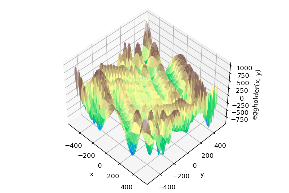
全域最佳化的目標是在給定邊界內找到函數的全域最小值，在可能存在許多局部最小值的情況下。 通常，全域最小化器會有效率地搜尋參數空間，同時在底層使用局部最小化器 (例如，minimize)。 SciPy 包含許多良好的全域最佳化器。 在此，我們將在相同的目標函數上使用它們，即（恰如其名）eggholder 函數

>>> def eggholder(x):
...     return (-(x[1] + 47) * np.sin(np.sqrt(abs(x[0]/2 + (x[1]  + 47))))
...             -x[0] * np.sin(np.sqrt(abs(x[0] - (x[1]  + 47)))))

>>> bounds = [(-512, 512), (-512, 512)]

此函數看起來像蛋盒

>>> import matplotlib.pyplot as plt
>>> from mpl_toolkits.mplot3d import Axes3D

>>> x = np.arange(-512, 513)
>>> y = np.arange(-512, 513)
>>> xgrid, ygrid = np.meshgrid(x, y)
>>> xy = np.stack([xgrid, ygrid])

>>> fig = plt.figure()
>>> ax = fig.add_subplot(111, projection='3d')
>>> ax.view_init(45, -45)
>>> ax.plot_surface(xgrid, ygrid, eggholder(xy), cmap='terrain')
>>> ax.set_xlabel('x')
>>> ax.set_ylabel('y')
>>> ax.set_zlabel('eggholder(x, y)')
>>> plt.show()

我們現在使用全域最佳化器來取得最小值以及最小值時的函數值。 我們會將結果儲存在字典中，以便稍後比較不同的最佳化結果。

>>> from scipy import optimize
>>> results = dict()
>>> results['shgo'] = optimize.shgo(eggholder, bounds)
>>> results['shgo']
     fun: -935.3379515604197  # may vary
    funl: array([-935.33795156])
 message: 'Optimization terminated successfully.'
    nfev: 42
     nit: 2
   nlfev: 37
   nlhev: 0
   nljev: 9
 success: True
       x: array([439.48096952, 453.97740589])
      xl: array([[439.48096952, 453.97740589]])

>>> results['DA'] = optimize.dual_annealing(eggholder, bounds)
>>> results['DA']
     fun: -956.9182316237413  # may vary
 message: ['Maximum number of iteration reached']
    nfev: 4091
    nhev: 0
     nit: 1000
    njev: 0
       x: array([482.35324114, 432.87892901])

所有最佳化器都會傳回 OptimizeResult，除了解決方案之外，還包含函數評估次數、最佳化是否成功等資訊。 為了簡潔起見，我們不會顯示其他最佳化器的完整輸出

>>> results['DE'] = optimize.differential_evolution(eggholder, bounds)

shgo 有第二種方法，可以傳回所有局部最小值，而不僅僅是它認為的全域最小值

>>> results['shgo_sobol'] = optimize.shgo(eggholder, bounds, n=200, iters=5,
...                                       sampling_method='sobol')

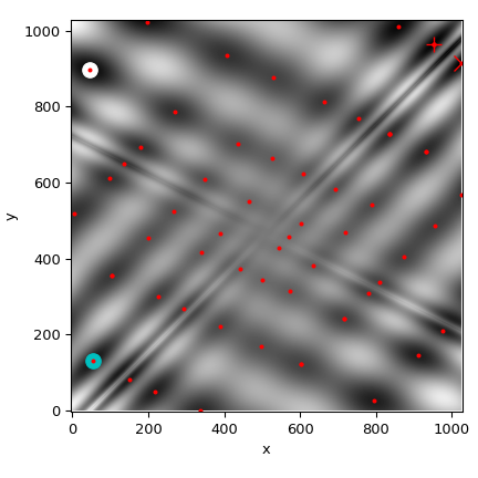
我們現在將所有找到的最小值繪製在函數的熱圖上

>>> fig = plt.figure()
>>> ax = fig.add_subplot(111)
>>> im = ax.imshow(eggholder(xy), interpolation='bilinear', origin='lower',
...                cmap='gray')
>>> ax.set_xlabel('x')
>>> ax.set_ylabel('y')
>>>
>>> def plot_point(res, marker='o', color=None):
...     ax.plot(512+res.x[0], 512+res.x[1], marker=marker, color=color, ms=10)

>>> plot_point(results['DE'], color='c')  # differential_evolution - cyan
>>> plot_point(results['DA'], color='w')  # dual_annealing.        - white

>>> # SHGO produces multiple minima, plot them all (with a smaller marker size)
>>> plot_point(results['shgo'], color='r', marker='+')
>>> plot_point(results['shgo_sobol'], color='r', marker='x')
>>> for i in range(results['shgo_sobol'].xl.shape[0]):
...     ax.plot(512 + results['shgo_sobol'].xl[i, 0],
...             512 + results['shgo_sobol'].xl[i, 1],
...             'ro', ms=2)

>>> ax.set_xlim([-4, 514*2])
>>> ax.set_ylim([-4, 514*2])
>>> plt.show()

全域最佳化器之比較

使用下表找到符合您需求的求解器。如果有多個候選者，請嘗試幾個，看看哪個最符合您的需求 (例如，執行時間、目標函數值)。

求解器	邊界約束	非線性約束	使用梯度	使用 Hessian
basinhopping			(✓)	(✓)
direct	✓
dual_annealing	✓		(✓)	(✓)
differential_evolution	✓	✓
shgo	✓	✓	(✓)	(✓)

(✓) = 取決於選擇的局部最小化器

最小平方法最小化 (least_squares)

SciPy 能夠解決穩健的有界限非線性最小平方法問題

\begin{align} &\min_\mathbf{x} \frac{1}{2} \sum_{i = 1}^m \rho\left(f_i(\mathbf{x})^2\right) \\ &\text{受限於 }\mathbf{lb} \leq \mathbf{x} \leq \mathbf{ub} \end{align}

此處 \(f_i(\mathbf{x})\) 是從 \(\mathbb{R}^n\) 到 \(\mathbb{R}\) 的平滑函數，我們將它們稱為殘差。 標量值函數 \(\rho(\cdot)\) 的目的是減少離群殘差的影響，並有助於解的穩健性，我們將其稱為損失函數。 線性損失函數會產生標準的最小平方法問題。 此外，允許對某些 \(x_j\) 施加下限和上限形式的約束。

最小平方法最小化的所有特定方法都使用 \(m \times n\) 的偏導數矩陣，稱為 Jacobian，定義為 \(J_{ij} = \partial f_i / \partial x_j\)。 強烈建議以解析方式計算此矩陣並將其傳遞給 least_squares，否則，它將透過有限差分法估算，這會花費大量額外時間，並且在困難情況下可能非常不準確。

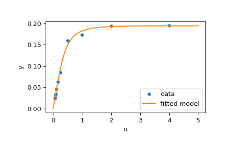
函數 least_squares 可用於將函數 \(\varphi(t; \mathbf{x})\) 擬合到經驗資料 \(\{(t_i, y_i), i = 0, \ldots, m-1\}\)。 若要執行此操作，應簡單地預先計算殘差為 \(f_i(\mathbf{x}) = w_i (\varphi(t_i; \mathbf{x}) - y_i)\)，其中 \(w_i\) 是指派給每個觀察值的權重。

求解擬合問題範例

在此，我們考慮酶促反應 [1]。 有 11 個殘差定義為

\[f_i(x) = \frac{x_0 (u_i^2 + u_i x_1)}{u_i^2 + u_i x_2 + x_3} - y_i, \quad i = 0, \ldots, 10,\]

其中 \(y_i\) 是測量值，而 \(u_i\) 是自變數的值。 未知參數向量為 \(\mathbf{x} = (x_0, x_1, x_2, x_3)^T\)。 如先前所述，建議以封閉形式計算 Jacobian 矩陣

\begin{align} &J_{i0} = \frac{\partial f_i}{\partial x_0} = \frac{u_i^2 + u_i x_1}{u_i^2 + u_i x_2 + x_3} \\ &J_{i1} = \frac{\partial f_i}{\partial x_1} = \frac{u_i x_0}{u_i^2 + u_i x_2 + x_3} \\ &J_{i2} = \frac{\partial f_i}{\partial x_2} = -\frac{x_0 (u_i^2 + u_i x_1) u_i}{(u_i^2 + u_i x_2 + x_3)^2} \\ &J_{i3} = \frac{\partial f_i}{\partial x_3} = -\frac{x_0 (u_i^2 + u_i x_1)}{(u_i^2 + u_i x_2 + x_3)^2} \end{align}

我們將使用 [2] 中定義的「困難」起點。 為了找到具有物理意義的解，避免潛在的除以零，並確保收斂到全域最小值，我們施加約束 \(0 \leq x_j \leq 100, j = 0, 1, 2, 3\)。

下面的程式碼實作了 \(\mathbf{x}\) 的最小平方法估計，並最終繪製原始資料和擬合模型函數

>>> from scipy.optimize import least_squares

>>> def model(x, u):
...     return x[0] * (u ** 2 + x[1] * u) / (u ** 2 + x[2] * u + x[3])

>>> def fun(x, u, y):
...     return model(x, u) - y

>>> def jac(x, u, y):
...     J = np.empty((u.size, x.size))
...     den = u ** 2 + x[2] * u + x[3]
...     num = u ** 2 + x[1] * u
...     J[:, 0] = num / den
...     J[:, 1] = x[0] * u / den
...     J[:, 2] = -x[0] * num * u / den ** 2
...     J[:, 3] = -x[0] * num / den ** 2
...     return J

>>> u = np.array([4.0, 2.0, 1.0, 5.0e-1, 2.5e-1, 1.67e-1, 1.25e-1, 1.0e-1,
...               8.33e-2, 7.14e-2, 6.25e-2])
>>> y = np.array([1.957e-1, 1.947e-1, 1.735e-1, 1.6e-1, 8.44e-2, 6.27e-2,
...               4.56e-2, 3.42e-2, 3.23e-2, 2.35e-2, 2.46e-2])
>>> x0 = np.array([2.5, 3.9, 4.15, 3.9])
>>> res = least_squares(fun, x0, jac=jac, bounds=(0, 100), args=(u, y), verbose=1)
# may vary
`ftol` termination condition is satisfied.
Function evaluations 130, initial cost 4.4383e+00, final cost 1.5375e-04, first-order optimality 4.92e-08.
>>> res.x
array([ 0.19280596,  0.19130423,  0.12306063,  0.13607247])

>>> import matplotlib.pyplot as plt
>>> u_test = np.linspace(0, 5)
>>> y_test = model(res.x, u_test)
>>> plt.plot(u, y, 'o', markersize=4, label='data')
>>> plt.plot(u_test, y_test, label='fitted model')
>>> plt.xlabel("u")
>>> plt.ylabel("y")
>>> plt.legend(loc='lower right')
>>> plt.show()

[1]

J. Kowalik 和 J. F. Morrison，「Analysis of kinetic data for allosteric enzyme reactions as a nonlinear regression problem」，Math. Biosci.，第 2 卷，第 57-66 頁，1968 年。

[2]

2. 13. Averick 等人，「The MINPACK-2 Test Problem Collection」。

更多範例

以下三個互動式範例說明了 least_squares 的更詳細用法。

1. scipy 中的大規模集束調整 示範了 least_squares 的大規模功能，以及如何有效率地計算稀疏 Jacobian 的有限差分近似值。

2. scipy 中的穩健非線性迴歸 說明如何在非線性迴歸中使用穩健損失函數處理離群值。

3. scipy 中求解離散邊界值問題 檢視如何求解大型方程式系統，並使用邊界來達成解的所需屬性。

有關實作背後的數學演算法的詳細資訊，請參閱 least_squares 的文件。

單變數函數最小化器 (minimize_scalar)

通常只需要單變數函數（即，將純量作為輸入的函數）的最小值。 在這些情況下，已開發出其他可以更快運作的最佳化技術。 這些可以從 minimize_scalar 函數存取，該函數提出了幾種演算法。

無約束最小化 (method='brent')

實際上，有兩種方法可用於最小化單變數函數：brent 和 golden，但 golden 僅出於學術目的而包含，應極少使用。 這些可以分別透過 minimize_scalar 中的 method 參數選取。 brent 方法使用 Brent 演算法來定位最小值。 最佳情況是，應給出包含所需最小值的括號（bracket 參數）。 括號是三元組 \(\left( a, b, c \right)\)，使得 \(f \left( a \right) > f \left( b \right) < f \left( c \right)\) 且 \(a < b < c\)。 如果未給出，則可以選擇兩個起點，並使用簡單的行進演算法從這些點找到括號。 如果未提供這兩個起點，則將使用 0 和 1（這可能不是您函數的正確選擇，並導致傳回意外的最小值）。

這是一個範例

>>> from scipy.optimize import minimize_scalar
>>> f = lambda x: (x - 2) * (x + 1)**2
>>> res = minimize_scalar(f, method='brent')
>>> print(res.x)
1.0

有界限最小化 (method='bounded')

通常，在進行最小化之前，可以對解空間施加約束。 minimize_scalar 中的 bounded 方法是約束最小化程序的一個範例，它為純量函數提供基本的間隔約束。 間隔約束允許最小化僅在兩個固定端點之間發生，這些端點使用強制性的 bounds 參數指定。

例如，若要找到 \(J_{1}\left( x \right)\) 在 \(x=5\) 附近的最小值，可以使用間隔 \(\left[ 4, 7 \right]\) 作為約束來呼叫 minimize_scalar。 結果為 \(x_{\textrm{min}}=5.3314\)

>>> from scipy.special import j1
>>> res = minimize_scalar(j1, bounds=(4, 7), method='bounded')
>>> res.x
5.33144184241

自訂最小化器

有時，使用自訂方法作為（多變數或單變數）最小化器可能很有用，例如，在使用 minimize 的某些程式庫包裝函式時（例如，basinhopping）。

我們可以透過傳遞可呼叫物件（函數或實作 __call__ 方法的物件）作為 method 參數，而不是傳遞方法名稱來實現此目的。

讓我們考慮一個（誠然相當虛擬的）需求，即使用一個簡單的自訂多變數最小化方法，該方法將僅以固定的步長獨立地搜尋每個維度中的鄰域

>>> from scipy.optimize import OptimizeResult
>>> def custmin(fun, x0, args=(), maxfev=None, stepsize=0.1,
...         maxiter=100, callback=None, **options):
...     bestx = x0
...     besty = fun(x0)
...     funcalls = 1
...     niter = 0
...     improved = True
...     stop = False
...
...     while improved and not stop and niter < maxiter:
...         improved = False
...         niter += 1
...         for dim in range(np.size(x0)):
...             for s in [bestx[dim] - stepsize, bestx[dim] + stepsize]:
...                 testx = np.copy(bestx)
...                 testx[dim] = s
...                 testy = fun(testx, *args)
...                 funcalls += 1
...                 if testy < besty:
...                     besty = testy
...                     bestx = testx
...                     improved = True
...             if callback is not None:
...                 callback(bestx)
...             if maxfev is not None and funcalls >= maxfev:
...                 stop = True
...                 break
...
...     return OptimizeResult(fun=besty, x=bestx, nit=niter,
...                           nfev=funcalls, success=(niter > 1))
>>> x0 = [1.35, 0.9, 0.8, 1.1, 1.2]
>>> res = minimize(rosen, x0, method=custmin, options=dict(stepsize=0.05))
>>> res.x
array([1., 1., 1., 1., 1.])

這在單變數最佳化的情況下也能很好地運作

>>> def custmin(fun, bracket, args=(), maxfev=None, stepsize=0.1,
...         maxiter=100, callback=None, **options):
...     bestx = (bracket[1] + bracket[0]) / 2.0
...     besty = fun(bestx)
...     funcalls = 1
...     niter = 0
...     improved = True
...     stop = False
...
...     while improved and not stop and niter < maxiter:
...         improved = False
...         niter += 1
...         for testx in [bestx - stepsize, bestx + stepsize]:
...             testy = fun(testx, *args)
...             funcalls += 1
...             if testy < besty:
...                 besty = testy
...                 bestx = testx
...                 improved = True
...         if callback is not None:
...             callback(bestx)
...         if maxfev is not None and funcalls >= maxfev:
...             stop = True
...             break
...
...     return OptimizeResult(fun=besty, x=bestx, nit=niter,
...                           nfev=funcalls, success=(niter > 1))
>>> def f(x):
...    return (x - 2)**2 * (x + 2)**2
>>> res = minimize_scalar(f, bracket=(-3.5, 0), method=custmin,
...                       options=dict(stepsize = 0.05))
>>> res.x
-2.0

求根

純量函數

如果有一個單變數方程式，則可以嘗試多種不同的求根演算法。 這些演算法中的大多數需要預期根所在的區間的端點（因為函數會變號）。 一般而言，brentq 是最佳選擇，但其他方法在某些情況下或出於學術目的可能很有用。 當括號不可用，但一個或多個導數可用時，則 newton（或 halley、secant）可能適用。 如果函數定義在複數平面的子集上，並且無法使用括號方法，則尤其如此。

定點求解

與尋找函數的零點密切相關的問題是尋找函數的定點的問題。 函數的定點是函數評估傳回該點的點：\(g\left(x\right)=x.\) 顯然，\(g\) 的定點是 \(f\left(x\right)=g\left(x\right)-x.\) 的根。 相同地，\(f\) 的根是 \(g\left(x\right)=f\left(x\right)+x.\) 的定點。 常式 fixed_point 提供了一種使用 Aitkens 序列加速的簡單迭代方法，以估計給定起點的 \(g\) 的定點。

方程式組

可以使用 root 函數找到一組非線性方程式的根。 有幾種方法可用，其中包括 hybr（預設值）和 lm，它們分別使用 Powell 的混合方法和 MINPACK 的 Levenberg-Marquardt 方法。

以下範例考慮單變數超越方程式

\[x+2\cos\left(x\right)=0,\]

可以找到其根，如下所示

>>> import numpy as np
>>> from scipy.optimize import root
>>> def func(x):
...     return x + 2 * np.cos(x)
>>> sol = root(func, 0.3)
>>> sol.x
array([-1.02986653])
>>> sol.fun
array([ -6.66133815e-16])

現在考慮一組非線性方程式

\begin{eqnarray*} x_{0}\cos\left(x_{1}\right) & = & 4,\\ x_{0}x_{1}-x_{1} & = & 5. \end{eqnarray*}

我們定義目標函數，使其也傳回 Jacobian，並透過將 jac 參數設定為 True 來指示這一點。 此外，此處使用了 Levenberg-Marquardt 求解器。

>>> def func2(x):
...     f = [x[0] * np.cos(x[1]) - 4,
...          x[1]*x[0] - x[1] - 5]
...     df = np.array([[np.cos(x[1]), -x[0] * np.sin(x[1])],
...                    [x[1], x[0] - 1]])
...     return f, df
>>> sol = root(func2, [1, 1], jac=True, method='lm')
>>> sol.x
array([ 6.50409711,  0.90841421])

大型問題的求根

root 中的方法 hybr 和 lm 無法處理非常大量的變數 (N)，因為它們需要在每個 Newton 步驟中計算並反轉密集的 N x N Jacobian 矩陣。 當 N 成長時，這變得相當沒有效率。

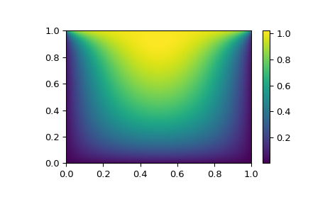
例如，考慮以下問題：我們需要在正方形 \([0,1]\times[0,1]\) 上求解以下積分微分方程式

\[(\partial_x^2 + \partial_y^2) P + 5 \left(\int_0^1\int_0^1\cosh(P)\,dx\,dy\right)^2 = 0\]

邊界條件為在上邊緣的 \(P(x,1) = 1\) 和正方形邊界上其他位置的 \(P=0\)。 這可以透過以網格上的值 \(P_{n,m}\approx{}P(n h, m h)\) 近似連續函數 P 來完成，其中網格間距 h 很小。 然後可以近似導數和積分； 例如 \(\partial_x^2 P(x,y)\approx{}(P(x+h,y) - 2 P(x,y) + P(x-h,y))/h^2\)。 然後問題等效於找到某些函數 residual(P) 的根，其中 P 是長度為 \(N_x N_y\) 的向量。

現在，由於 \(N_x N_y\) 可能很大，因此 root 中的方法 hybr 或 lm 將花費很長時間來解決此問題。 但是，可以使用大型求解器之一找到解，例如 krylov、broyden2 或 anderson。 這些使用所謂的不精確 Newton 方法，該方法不是精確計算 Jacobian 矩陣，而是形成其近似值。

我們現在可以按如下方式解決我們遇到的問題

import numpy as np
from scipy.optimize import root
from numpy import cosh, zeros_like, mgrid, zeros

# parameters
nx, ny = 75, 75
hx, hy = 1./(nx-1), 1./(ny-1)

P_left, P_right = 0, 0
P_top, P_bottom = 1, 0

def residual(P):
   d2x = zeros_like(P)
   d2y = zeros_like(P)

   d2x[1:-1] = (P[2:]   - 2*P[1:-1] + P[:-2]) / hx/hx
   d2x[0]    = (P[1]    - 2*P[0]    + P_left)/hx/hx
   d2x[-1]   = (P_right - 2*P[-1]   + P[-2])/hx/hx

   d2y[:,1:-1] = (P[:,2:] - 2*P[:,1:-1] + P[:,:-2])/hy/hy
   d2y[:,0]    = (P[:,1]  - 2*P[:,0]    + P_bottom)/hy/hy
   d2y[:,-1]   = (P_top   - 2*P[:,-1]   + P[:,-2])/hy/hy

   return d2x + d2y + 5*cosh(P).mean()**2

# solve
guess = zeros((nx, ny), float)
sol = root(residual, guess, method='krylov', options={'disp': True})
#sol = root(residual, guess, method='broyden2', options={'disp': True, 'max_rank': 50})
#sol = root(residual, guess, method='anderson', options={'disp': True, 'M': 10})
print('Residual: %g' % abs(residual(sol.x)).max())

# visualize
import matplotlib.pyplot as plt
x, y = mgrid[0:1:(nx*1j), 0:1:(ny*1j)]
plt.pcolormesh(x, y, sol.x, shading='gouraud')
plt.colorbar()
plt.show()

仍然太慢？ 預處理。

在尋找函數 \(f_i({\bf x}) = 0\)，i = 1, 2, …, N 的零點時，krylov 求解器將大部分時間花費在反轉 Jacobian 矩陣上，

\[J_{ij} = \frac{\partial f_i}{\partial x_j} .\]

如果您有逆矩陣 \(M\approx{}J^{-1}\) 的近似值，則可以使用它來預處理線性反轉問題。 其想法是，不是求解 \(J{\bf s}={\bf y}\)，而是求解 \(MJ{\bf s}=M{\bf y}\)：由於矩陣 \(MJ\) 比 \(J\)「更接近」單位矩陣，因此方程式對於 Krylov 方法來說應該更容易處理。

矩陣 M 可以透過選項 options['jac_options']['inner_M'] 與方法 krylov 一起傳遞給 root。 它可以是（稀疏）矩陣或 scipy.sparse.linalg.LinearOperator 實例。

對於上一節中的問題，我們注意到要解決的函數包含兩個部分：第一部分是 Laplace 算子的應用，\([\partial_x^2 + \partial_y^2] P\)，第二部分是積分。 我們實際上可以輕鬆計算對應於 Laplace 算子部分的 Jacobian：我們知道在 1-D 中

\[\begin{split}\partial_x^2 \approx \frac{1}{h_x^2} \begin{pmatrix} -2 & 1 & 0 & 0 \cdots \\ 1 & -2 & 1 & 0 \cdots \\ 0 & 1 & -2 & 1 \cdots \\ \ldots \end{pmatrix} = h_x^{-2} L\end{split}\]

因此，整個 2-D 算子由下式表示

\[J_1 = \partial_x^2 + \partial_y^2 \simeq h_x^{-2} L \otimes I + h_y^{-2} I \otimes L\]

與積分對應的 Jacobian 矩陣 \(J_2\) 更難計算，並且由於它的所有條目都非零，因此很難反轉。 另一方面，\(J_1\) 是一個相對簡單的矩陣，可以透過 scipy.sparse.linalg.splu 反轉（或者逆矩陣可以透過 scipy.sparse.linalg.spilu 近似）。 因此，我們滿足於取 \(M\approx{}J_1^{-1}\) 並期待最好的結果。

在下面的範例中，我們使用預處理器 \(M=J_1^{-1}\)。

from scipy.optimize import root
from scipy.sparse import dia_array, kron
from scipy.sparse.linalg import spilu, LinearOperator
from numpy import cosh, zeros_like, mgrid, zeros, eye

# parameters
nx, ny = 75, 75
hx, hy = 1./(nx-1), 1./(ny-1)

P_left, P_right = 0, 0
P_top, P_bottom = 1, 0

def get_preconditioner():
    """Compute the preconditioner M"""
    diags_x = zeros((3, nx))
    diags_x[0,:] = 1/hx/hx
    diags_x[1,:] = -2/hx/hx
    diags_x[2,:] = 1/hx/hx
    Lx = dia_array((diags_x, [-1,0,1]), shape=(nx, nx))

    diags_y = zeros((3, ny))
    diags_y[0,:] = 1/hy/hy
    diags_y[1,:] = -2/hy/hy
    diags_y[2,:] = 1/hy/hy
    Ly = dia_array((diags_y, [-1,0,1]), shape=(ny, ny))

    J1 = kron(Lx, eye(ny)) + kron(eye(nx), Ly)

    # Now we have the matrix `J_1`. We need to find its inverse `M` --
    # however, since an approximate inverse is enough, we can use
    # the *incomplete LU* decomposition

    J1_ilu = spilu(J1)

    # This returns an object with a method .solve() that evaluates
    # the corresponding matrix-vector product. We need to wrap it into
    # a LinearOperator before it can be passed to the Krylov methods:

    M = LinearOperator(shape=(nx*ny, nx*ny), matvec=J1_ilu.solve)
    return M

def solve(preconditioning=True):
    """Compute the solution"""
    count = [0]

    def residual(P):
        count[0] += 1

        d2x = zeros_like(P)
        d2y = zeros_like(P)

        d2x[1:-1] = (P[2:]   - 2*P[1:-1] + P[:-2])/hx/hx
        d2x[0]    = (P[1]    - 2*P[0]    + P_left)/hx/hx
        d2x[-1]   = (P_right - 2*P[-1]   + P[-2])/hx/hx

        d2y[:,1:-1] = (P[:,2:] - 2*P[:,1:-1] + P[:,:-2])/hy/hy
        d2y[:,0]    = (P[:,1]  - 2*P[:,0]    + P_bottom)/hy/hy
        d2y[:,-1]   = (P_top   - 2*P[:,-1]   + P[:,-2])/hy/hy

        return d2x + d2y + 5*cosh(P).mean()**2

    # preconditioner
    if preconditioning:
        M = get_preconditioner()
    else:
        M = None

    # solve
    guess = zeros((nx, ny), float)

    sol = root(residual, guess, method='krylov',
               options={'disp': True,
                        'jac_options': {'inner_M': M}})
    print('Residual', abs(residual(sol.x)).max())
    print('Evaluations', count[0])

    return sol.x

def main():
    sol = solve(preconditioning=True)

    # visualize
    import matplotlib.pyplot as plt
    x, y = mgrid[0:1:(nx*1j), 0:1:(ny*1j)]
    plt.clf()
    plt.pcolor(x, y, sol)
    plt.clim(0, 1)
    plt.colorbar()
    plt.show()


if __name__ == "__main__":
    main()

產生的執行，首先不使用預處理

0:  |F(x)| = 803.614; step 1; tol 0.000257947
1:  |F(x)| = 345.912; step 1; tol 0.166755
2:  |F(x)| = 139.159; step 1; tol 0.145657
3:  |F(x)| = 27.3682; step 1; tol 0.0348109
4:  |F(x)| = 1.03303; step 1; tol 0.00128227
5:  |F(x)| = 0.0406634; step 1; tol 0.00139451
6:  |F(x)| = 0.00344341; step 1; tol 0.00645373
7:  |F(x)| = 0.000153671; step 1; tol 0.00179246
8:  |F(x)| = 6.7424e-06; step 1; tol 0.00173256
Residual 3.57078908664e-07
Evaluations 317

然後使用預處理

0:  |F(x)| = 136.993; step 1; tol 7.49599e-06
1:  |F(x)| = 4.80983; step 1; tol 0.00110945
2:  |F(x)| = 0.195942; step 1; tol 0.00149362
3:  |F(x)| = 0.000563597; step 1; tol 7.44604e-06
4:  |F(x)| = 1.00698e-09; step 1; tol 2.87308e-12
Residual 9.29603061195e-11
Evaluations 77

使用預處理器將 residual 函數的評估次數減少了 4 倍。 對於殘差計算成本高昂的問題，良好的預處理至關重要 — 它甚至可以決定問題在實務上是否可解。

預處理是一門藝術、科學和產業。 在此，我們很幸運地做出了一個簡單的選擇，效果相當不錯，但這個主題比此處所示的更深入。

線性規劃 (linprog)

函數 linprog 可以最小化受線性等式和不等式約束的線性目標函數。 這種問題眾所周知為線性規劃。 線性規劃解決以下形式的問題

\[\begin{split}\min_x \ & c^T x \\ \mbox{受限於} \ & A_{ub} x \leq b_{ub},\\ & A_{eq} x = b_{eq},\\ & l \leq x \leq u ,\end{split}\]

其中 \(x\) 是決策變數的向量； \(c\)、\(b_{ub}\)、\(b_{eq}\)、\(l\) 和 \(u\) 是向量； 而 \(A_{ub}\) 和 \(A_{eq}\) 是矩陣。

在本教學課程中，我們將嘗試使用 linprog 解決典型的線性規劃問題。

線性規劃範例

考慮以下簡單的線性規劃問題

\[\begin{split}\max_{x_1, x_2, x_3, x_4} \ & 29x_1 + 45x_2 \\ \mbox{受限於} \ & x_1 -x_2 -3x_3 \leq 5\\ & 2x_1 -3x_2 -7x_3 + 3x_4 \geq 10\\ & 2x_1 + 8x_2 + x_3 = 60\\ & 4x_1 + 4x_2 + x_4 = 60\\ & 0 \leq x_0\\ & 0 \leq x_1 \leq 5\\ & x_2 \leq 0.5\\ & -3 \leq x_3\\\end{split}\]

我們需要進行一些數學運算，才能將目標問題轉換為 linprog 接受的形式。

首先，讓我們考慮目標函數。 我們想要最大化目標函數，但 linprog 只能接受最小化問題。 這很容易透過將最大化 \(29x_1 + 45x_2\) 轉換為最小化 \(-29x_1 -45x_2\) 來補救。 此外，\(x_3, x_4\) 未顯示在目標函數中。 這表示與 \(x_3, x_4\) 對應的權重為零。 因此，目標函數可以轉換為

\[\min_{x_1, x_2, x_3, x_4} \ -29x_1 -45x_2 + 0x_3 + 0x_4\]

如果我們定義決策變數向量 \(x = [x_1, x_2, x_3, x_4]^T\)，則此問題中 linprog 的目標權重向量 \(c\) 應為

\[c = [-29, -45, 0, 0]^T\]

接下來，讓我們考慮兩個不等式約束。 第一個是「小於」不等式，因此它已經是 linprog 接受的形式。 第二個是「大於」不等式，因此我們需要將兩邊都乘以 \(-1\) 以將其轉換為「小於」不等式。 明確顯示零係數，我們有

\[\begin{split}x_1 -x_2 -3x_3 + 0x_4 &\leq 5\\ -2x_1 + 3x_2 + 7x_3 - 3x_4 &\leq -10\\\end{split}\]

這些方程式可以轉換為矩陣形式

\[\begin{split}A_{ub} x \leq b_{ub}\\\end{split}\]

其中

\begin{equation*} A_{ub} = \begin{bmatrix} 1 & -1 & -3 & 0 \\ -2 & 3 & 7 & -3 \end{bmatrix} \end{equation*}

\begin{equation*} b_{ub} = \begin{bmatrix} 5 \\ -10 \end{bmatrix} \end{equation*}

接下來，讓我們考慮兩個等式約束。 明確顯示零權重，這些是

\[\begin{split}2x_1 + 8x_2 + 1x_3 + 0x_4 &= 60\\ 4x_1 + 4x_2 + 0x_3 + 1x_4 &= 60\\\end{split}\]

這些方程式可以轉換為矩陣形式

\[\begin{split}A_{eq} x = b_{eq}\\\end{split}\]

其中

\begin{equation*} A_{eq} = \begin{bmatrix} 2 & 8 & 1 & 0 \\ 4 & 4 & 0 & 1 \end{bmatrix} \end{equation*}

\begin{equation*} b_{eq} = \begin{bmatrix} 60 \\ 60 \end{bmatrix} \end{equation*}

最後，讓我們考慮對個別決策變數的單獨不等式約束，這些約束稱為「方塊約束」或「簡單邊界」。 這些約束可以使用 linprog 的 bounds 引數套用。 如 linprog 文件中所述，bounds 的預設值為 (0, None)，表示每個決策變數的下限為 0，而每個決策變數的上限為無限大：所有決策變數均為非負數。 我們的邊界不同，因此我們需要將每個決策變數的下限和上限指定為元組，並將這些元組分組到清單中。

最後，我們可以使用 linprog 求解轉換後的問題。

>>> import numpy as np
>>> from scipy.optimize import linprog
>>> c = np.array([-29.0, -45.0, 0.0, 0.0])
>>> A_ub = np.array([[1.0, -1.0, -3.0, 0.0],
...                 [-2.0, 3.0, 7.0, -3.0]])
>>> b_ub = np.array([5.0, -10.0])
>>> A_eq = np.array([[2.0, 8.0, 1.0, 0.0],
...                 [4.0, 4.0, 0.0, 1.0]])
>>> b_eq = np.array([60.0, 60.0])
>>> x0_bounds = (0, None)
>>> x1_bounds = (0, 5.0)
>>> x2_bounds = (-np.inf, 0.5)  # +/- np.inf can be used instead of None
>>> x3_bounds = (-3.0, None)
>>> bounds = [x0_bounds, x1_bounds, x2_bounds, x3_bounds]
>>> result = linprog(c, A_ub=A_ub, b_ub=b_ub, A_eq=A_eq, b_eq=b_eq, bounds=bounds)
>>> print(result.message)
The problem is infeasible. (HiGHS Status 8: model_status is Infeasible; primal_status is None)

結果指出我們的問題不可行，表示沒有任何解決方案向量可以滿足所有約束。 這不一定表示我們做錯了任何事； 有些問題確實不可行。 但是，假設我們決定對 \(x_1\) 的邊界約束太嚴格，並且可以放寬到 \(0 \leq x_1 \leq 6\)。 在調整我們的程式碼 x1_bounds = (0, 6) 以反映變更並再次執行它之後

>>> x1_bounds = (0, 6)
>>> bounds = [x0_bounds, x1_bounds, x2_bounds, x3_bounds]
>>> result = linprog(c, A_ub=A_ub, b_ub=b_ub, A_eq=A_eq, b_eq=b_eq, bounds=bounds)
>>> print(result.message)
Optimization terminated successfully. (HiGHS Status 7: Optimal)

結果顯示最佳化成功。 我們可以檢查目標值 (result.fun) 是否與 \(c^Tx\) 相同

>>> x = np.array(result.x)
>>> obj = result.fun
>>> print(c @ x)
-505.97435889013434  # may vary
>>> print(obj)
-505.97435889013434  # may vary

我們也可以檢查是否在合理的容差範圍內滿足所有約束

>>> print(b_ub - (A_ub @ x).flatten())  # this is equivalent to result.slack
[ 6.52747190e-10, -2.26730279e-09]  # may vary
>>> print(b_eq - (A_eq @ x).flatten())  # this is equivalent to result.con
[ 9.78840831e-09, 1.04662945e-08]]  # may vary
>>> print([0 <= result.x[0], 0 <= result.x[1] <= 6.0, result.x[2] <= 0.5, -3.0 <= result.x[3]])
[True, True, True, True]

指派問題

線性總和指派問題範例

考慮為游泳混合式接力隊選拔學生的問題。 我們有一個表格，顯示五名學生每種游泳風格的時間

學生	仰式	蛙式	蝶式	自由式
A	43.5	47.1	48.4	38.2
B	45.5	42.1	49.6	36.8
C	43.4	39.1	42.1	43.2
D	46.5	44.1	44.5	41.2
E	46.3	47.8	50.4	37.2

我們需要為四種游泳風格中的每種風格選擇一名學生，以使總接力時間最小化。 這是一個典型的線性總和指派問題。 我們可以使用 linear_sum_assignment 來解決它。

線性總和指派問題是最著名的組合最佳化問題之一。給定一個「成本矩陣」\(C\)，問題是要選擇

• 從每一行中恰好選擇一個元素

• 且不從任何行中選擇多於一個元素

• 使得所選元素的總和最小化

換句話說，我們需要將每一行指派給一行，使得對應條目的總和最小化。

正式地說，令 \(X\) 為一個布林矩陣，其中 \(X[i,j] = 1\) 若且唯若第 \(i\) 行被指派給第 \(j\) 欄。那麼，最佳指派的成本為

\[\min \sum_i \sum_j C_{i,j} X_{i,j}\]

第一步是定義成本矩陣。在這個例子中，我們想要將每種游泳風格指派給一位學生。linear_sum_assignment 能夠將成本矩陣的每一行指派給一欄。因此，為了形成成本矩陣，上面的表格需要轉置，以便行對應於游泳風格，而欄對應於學生

>>> import numpy as np
>>> cost = np.array([[43.5, 45.5, 43.4, 46.5, 46.3],
...                  [47.1, 42.1, 39.1, 44.1, 47.8],
...                  [48.4, 49.6, 42.1, 44.5, 50.4],
...                  [38.2, 36.8, 43.2, 41.2, 37.2]])

我們可以使用 linear_sum_assignment 來解決指派問題

>>> from scipy.optimize import linear_sum_assignment
>>> row_ind, col_ind = linear_sum_assignment(cost)

row_ind 和 col_ind 是成本矩陣的最佳指派矩陣索引

>>> row_ind
array([0, 1, 2, 3])
>>> col_ind
array([0, 2, 3, 1])

最佳指派是

>>> styles = np.array(["backstroke", "breaststroke", "butterfly", "freestyle"])[row_ind]
>>> students = np.array(["A", "B", "C", "D", "E"])[col_ind]
>>> dict(zip(styles, students))
{'backstroke': 'A', 'breaststroke': 'C', 'butterfly': 'D', 'freestyle': 'B'}

最佳總混合時間是

>>> cost[row_ind, col_ind].sum()
163.89999999999998

請注意，此結果與每種游泳風格的最小時間總和不同

>>> np.min(cost, axis=1).sum()
161.39999999999998

因為學生「C」是「蛙泳」和「蝶泳」風格中最好的游泳者。我們不能將學生「C」指派給兩種風格，所以我們將學生 C 指派給「蛙泳」風格，將 D 指派給「蝶泳」風格，以最小化總時間。

參考文獻

一些延伸閱讀和相關軟體，例如 Newton-Krylov [KK]、PETSc [PP] 和 PyAMG [AMG]

[KK]

D.A. Knoll 和 D.E. Keyes，「Jacobian-free Newton-Krylov methods」，J. Comp. Phys. 193, 357 (2004)。 DOI:10.1016/j.jcp.2003.08.010

[PP]

PETSc https://www.mcs.anl.gov/petsc/ 及其 Python 綁定 https://bitbucket.org/petsc/petsc4py/

[AMG]

PyAMG (代數多重網格預處理器/求解器) pyamg/pyamg#issues

混合整數線性規劃

背包問題範例

背包問題是一個著名的組合最佳化問題。給定一組物品，每件物品都有大小和價值，問題是要選擇在總大小低於特定閾值的情況下，最大化總價值的物品。

正式地說，令

• \(x_i\) 為一個布林變數，表示物品 \(i\) 是否包含在背包中，

• \(n\) 為物品總數，

• \(v_i\) 為物品 \(i\) 的價值，

• \(s_i\) 為物品 \(i\) 的大小，以及

• \(C\) 為背包的容量。

那麼問題是

\[\max \sum_i^n v_{i} x_{i}\]

\[\text{受限於} \sum_i^n s_{i} x_{i} \leq C, x_{i} \in {0, 1}\]

雖然目標函數和不等式約束在決策變數 \(x_i\) 中是線性的，但這與典型的線性規劃問題不同，因為決策變數只能假設整數值。具體而言，我們的決策變數只能是 \(0\) 或 \(1\)，因此這被稱為二元整數線性規劃 (BILP)。這類問題屬於更大的混合整數線性規劃 (MILP) 類別，我們可以使用 milp 來解決。

在我們的範例中，有 8 個物品可供選擇，每個物品的大小和價值如下所示。

>>> import numpy as np
>>> from scipy import optimize
>>> sizes = np.array([21, 11, 15, 9, 34, 25, 41, 52])
>>> values = np.array([22, 12, 16, 10, 35, 26, 42, 53])

我們需要約束我們的八個決策變數為二元的。我們通過添加 Bounds 約束來確保它們介於 \(0\) 和 \(1\) 之間，並且我們應用「整數性」約束來確保它們*是* \(0\) *或是* \(1\)。

>>> bounds = optimize.Bounds(0, 1)  # 0 <= x_i <= 1
>>> integrality = np.full_like(values, True)  # x_i are integers

背包容量約束是使用 LinearConstraint 指定的。

>>> capacity = 100
>>> constraints = optimize.LinearConstraint(A=sizes, lb=0, ub=capacity)

如果我們遵循線性代數的常用規則，則輸入 A 應該是一個二維矩陣，而下限和上限 lb 和 ub 應該是一維向量，但 LinearConstraint 是寬容的，只要輸入可以廣播到一致的形狀。

使用上面定義的變數，我們可以使用 milp 來解決背包問題。請注意，milp 最小化目標函數，但我們想要最大化總價值，因此我們將 c 設定為價值的負數。

>>> from scipy.optimize import milp
>>> res = milp(c=-values, constraints=constraints,
...            integrality=integrality, bounds=bounds)

讓我們檢查結果

>>> res.success
True
>>> res.x
array([1., 1., 0., 1., 1., 1., 0., 0.])

這表示我們應該選擇物品 1、2、4、5、6，以在大小約束下優化總價值。請注意，這與我們在解決線性規劃鬆弛（沒有整數性約束）並嘗試捨入決策變數時獲得的結果不同。

>>> from scipy.optimize import milp
>>> res = milp(c=-values, constraints=constraints,
...            integrality=False, bounds=bounds)
>>> res.x
array([1.        , 1.        , 1.        , 1.        ,
       0.55882353, 1.        , 0.        , 0.        ])

如果我們將此解決方案向上捨入到 array([1., 1., 1., 1., 1., 1., 0., 0.])，我們的背包將超過容量限制，而如果我們向下捨入到 array([1., 1., 1., 1., 0., 1., 0., 0.])，我們將得到一個次優解。

如需更多 MILP 教學，請參閱 SciPy Cookbooks 上的 Jupyter 筆記本

• Compressed Sensing l1 program

• Compressed Sensing l0 program