空間資料結構與演算法 (scipy.spatial)#
scipy.spatial 可以利用 Qhull 函式庫,計算一組點的三角剖分、Voronoi 圖和凸包。
此外,它還包含 KDTree 實作,用於最近鄰點查詢,以及用於各種度量中距離計算的工具。
Delaunay 三角剖分#
Delaunay 三角剖分是將一組點細分為一組不重疊的三角形,使得沒有點位於任何三角形的外接圓內。實際上,這種三角剖分傾向於避免小角度的三角形。
Delaunay 三角剖分可以使用 scipy.spatial 如下計算
>>> from scipy.spatial import Delaunay
>>> import numpy as np
>>> points = np.array([[0, 0], [0, 1.1], [1, 0], [1, 1]])
>>> tri = Delaunay(points)
我們可以將其視覺化
>>> import matplotlib.pyplot as plt
>>> plt.triplot(points[:,0], points[:,1], tri.simplices)
>>> plt.plot(points[:,0], points[:,1], 'o')
並添加一些進一步的裝飾
>>> for j, p in enumerate(points):
...     plt.text(p[0]-0.03, p[1]+0.03, j, ha='right') # label the points
>>> for j, s in enumerate(tri.simplices):
...     p = points[s].mean(axis=0)
...     plt.text(p[0], p[1], '#%d' % j, ha='center') # label triangles
>>> plt.xlim(-0.5, 1.5); plt.ylim(-0.5, 1.5)
>>> plt.show()
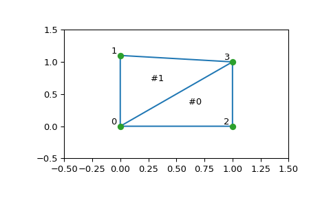
三角剖分的結構以下列方式編碼:simplices 屬性包含組成三角形的 points 陣列中點的索引。例如
>>> i = 1
>>> tri.simplices[i,:]
array([3, 1, 0], dtype=int32)
>>> points[tri.simplices[i,:]]
array([[ 1. ,  1. ],
       [ 0. ,  1.1],
       [ 0. ,  0. ]])
此外,也可以找到相鄰的三角形
>>> tri.neighbors[i]
array([-1,  0, -1], dtype=int32)
這告訴我們,這個三角形以三角形 #0 作為鄰居,但沒有其他鄰居。此外,它告訴我們鄰居 0 與三角形的頂點 1 相對
>>> points[tri.simplices[i, 1]]
array([ 0. ,  1.1])
實際上,從圖中我們可以看到情況確實如此。
Qhull 也可以對更高維度的點集執行單體鑲嵌(例如,在 3-D 中細分為四面體)。
共面點#
重要的是要注意,並非所有點都一定會作為三角剖分的頂點出現,這是由於形成三角剖分時的數值精度問題。考慮上面帶有重複點的情況
>>> points = np.array([[0, 0], [0, 1], [1, 0], [1, 1], [1, 1]])
>>> tri = Delaunay(points)
>>> np.unique(tri.simplices.ravel())
array([0, 1, 2, 3], dtype=int32)
請注意,點 #4(它是重複點)不會作為三角剖分的頂點出現。這種情況的發生已被記錄
>>> tri.coplanar
array([[4, 0, 3]], dtype=int32)
這表示點 4 位於三角形 0 和頂點 3 附近,但不包含在三角剖分中。
請注意,這種退化不僅可能由於重複點而發生,也可能由於更複雜的幾何原因而發生,即使在乍看之下行為良好的點集中也是如此。
但是,Qhull 具有 “QJ” 選項,它指示它隨機擾動輸入資料,直到退化得到解決
>>> tri = Delaunay(points, qhull_options="QJ Pp")
>>> points[tri.simplices]
array([[[1, 0],
        [1, 1],
        [0, 0]],
       [[1, 1],
        [1, 1],
        [1, 0]],
       [[1, 1],
        [0, 1],
        [0, 0]],
       [[0, 1],
        [1, 1],
        [1, 1]]])
出現了兩個新的三角形。但是,我們看到它們是退化的並且面積為零。
凸包#
凸包是包含給定點集中所有點的最小凸物件。
這些可以透過 scipy.spatial 中的 Qhull 包裝器計算如下
>>> from scipy.spatial import ConvexHull
>>> rng = np.random.default_rng()
>>> points = rng.random((30, 2))   # 30 random points in 2-D
>>> hull = ConvexHull(points)
凸包表示為一組 N 1-D 單體,在 2-D 中表示線段。儲存方案與上面討論的 Delaunay 三角剖分中的單體完全相同。
我們可以說明上面的結果
>>> import matplotlib.pyplot as plt
>>> plt.plot(points[:,0], points[:,1], 'o')
>>> for simplex in hull.simplices:
...     plt.plot(points[simplex,0], points[simplex,1], 'k-')
>>> plt.show()
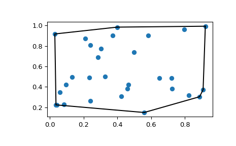
使用 scipy.spatial.convex_hull_plot_2d 也可以實現相同的效果。
Voronoi 圖#
Voronoi 圖是將空間細分為給定點集最近鄰域的細分。
有兩種方法可以使用 scipy.spatial 來處理此物件。首先,可以使用 KDTree 來回答問題「哪個點最接近這個點」,並以這種方式定義區域
>>> from scipy.spatial import KDTree
>>> points = np.array([[0, 0], [0, 1], [0, 2], [1, 0], [1, 1], [1, 2],
...                    [2, 0], [2, 1], [2, 2]])
>>> tree = KDTree(points)
>>> tree.query([0.1, 0.1])
(0.14142135623730953, 0)
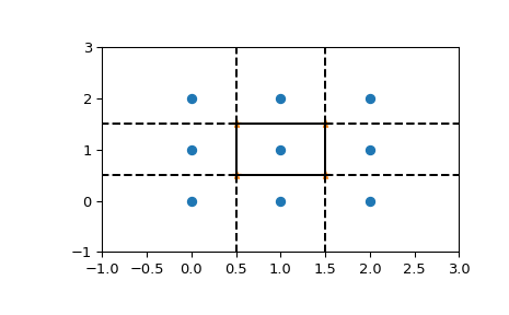
所以點 (0.1, 0.1) 屬於區域 0。以顏色表示
>>> x = np.linspace(-0.5, 2.5, 31)
>>> y = np.linspace(-0.5, 2.5, 33)
>>> xx, yy = np.meshgrid(x, y)
>>> xy = np.c_[xx.ravel(), yy.ravel()]
>>> import matplotlib.pyplot as plt
>>> dx_half, dy_half = np.diff(x[:2])[0] / 2., np.diff(y[:2])[0] / 2.
>>> x_edges = np.concatenate((x - dx_half, [x[-1] + dx_half]))
>>> y_edges = np.concatenate((y - dy_half, [y[-1] + dy_half]))
>>> plt.pcolormesh(x_edges, y_edges, tree.query(xy)[1].reshape(33, 31), shading='flat')
>>> plt.plot(points[:,0], points[:,1], 'ko')
>>> plt.show()
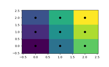
然而,這並未將 Voronoi 圖作為幾何物件給出。
線和點的表示可以再次透過 scipy.spatial 中的 Qhull 包裝器獲得
>>> from scipy.spatial import Voronoi
>>> vor = Voronoi(points)
>>> vor.vertices
array([[0.5, 0.5],
       [0.5, 1.5],
       [1.5, 0.5],
       [1.5, 1.5]])
Voronoi 頂點表示形成 Voronoi 區域多邊形邊緣的點集。在這種情況下,有 9 個不同的區域
>>> vor.regions
[[], [-1, 0], [-1, 1], [1, -1, 0], [3, -1, 2], [-1, 3], [-1, 2], [0, 1, 3, 2], [2, -1, 0], [3, -1, 1]]
負值 -1 再次表示無窮遠處的點。實際上,只有一個區域 [0, 1, 3, 2] 是有界的。這裡請注意,由於與上面 Delaunay 三角剖分中類似的數值精度問題,Voronoi 區域可能少於輸入點。
分隔區域的脊線(2-D 中的線)被描述為與凸包片段類似的單體集合
>>> vor.ridge_vertices
[[-1, 0], [-1, 0], [-1, 1], [-1, 1], [0, 1], [-1, 3], [-1, 2], [2, 3], [-1, 3], [-1, 2], [1, 3], [0, 2]]
這些數字表示構成線段的 Voronoi 頂點的索引。-1 再次是無窮遠處的點 — 12 條線中只有 4 條是有界線段,而其他線段延伸到無窮遠。
Voronoi 脊線垂直於在輸入點之間繪製的線。每個脊線對應於哪兩個點也被記錄下來
>>> vor.ridge_points
array([[0, 3],
       [0, 1],
       [2, 5],
       [2, 1],
       [1, 4],
       [7, 8],
       [7, 6],
       [7, 4],
       [8, 5],
       [6, 3],
       [4, 5],
       [4, 3]], dtype=int32)
將這些資訊放在一起,足以建構完整的圖。
我們可以按如下方式繪製它。首先,是點和 Voronoi 頂點
>>> plt.plot(points[:, 0], points[:, 1], 'o')
>>> plt.plot(vor.vertices[:, 0], vor.vertices[:, 1], '*')
>>> plt.xlim(-1, 3); plt.ylim(-1, 3)
繪製有限線段的方法與凸包相同,但現在我們必須注意無限邊緣
>>> for simplex in vor.ridge_vertices:
...     simplex = np.asarray(simplex)
...     if np.all(simplex >= 0):
...         plt.plot(vor.vertices[simplex, 0], vor.vertices[simplex, 1], 'k-')
延伸到無窮遠的脊線需要更多注意
>>> center = points.mean(axis=0)
>>> for pointidx, simplex in zip(vor.ridge_points, vor.ridge_vertices):
...     simplex = np.asarray(simplex)
...     if np.any(simplex < 0):
...         i = simplex[simplex >= 0][0] # finite end Voronoi vertex
...         t = points[pointidx[1]] - points[pointidx[0]]  # tangent
...         t = t / np.linalg.norm(t)
...         n = np.array([-t[1], t[0]]) # normal
...         midpoint = points[pointidx].mean(axis=0)
...         far_point = vor.vertices[i] + np.sign(np.dot(midpoint - center, n)) * n * 100
...         plt.plot([vor.vertices[i,0], far_point[0]],
...                  [vor.vertices[i,1], far_point[1]], 'k--')
>>> plt.show()
此圖也可以使用 scipy.spatial.voronoi_plot_2d 建立。
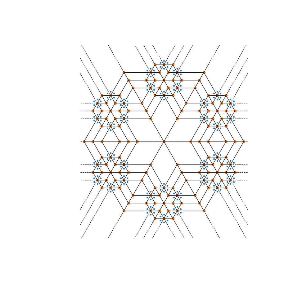
Voronoi 圖可用於創建有趣的生成藝術。嘗試調整此 mandala 函數的設定來創建您自己的作品!
>>> import numpy as np
>>> from scipy import spatial
>>> import matplotlib.pyplot as plt
>>> def mandala(n_iter, n_points, radius):
...     """Creates a mandala figure using Voronoi tessellations.
...
...     Parameters
...     ----------
...     n_iter : int
...         Number of iterations, i.e. how many times the equidistant points will
...         be generated.
...     n_points : int
...         Number of points to draw per iteration.
...     radius : scalar
...         The radial expansion factor.
...
...     Returns
...     -------
...     fig : matplotlib.Figure instance
...
...     Notes
...     -----
...     This code is adapted from the work of Audrey Roy Greenfeld [1]_ and Carlos
...     Focil-Espinosa [2]_, who created beautiful mandalas with Python code.  That
...     code in turn was based on Antonio Sánchez Chinchón's R code [3]_.
...
...     References
...     ----------
...     .. [1] https://www.codemakesmehappy.com/2019/09/voronoi-mandalas.html
...
...     .. [2] https://github.com/CarlosFocil/mandalapy
...
...     .. [3] https://github.com/aschinchon/mandalas
...
...     """
...     fig = plt.figure(figsize=(10, 10))
...     ax = fig.add_subplot(111)
...     ax.set_axis_off()
...     ax.set_aspect('equal', adjustable='box')
...
...     angles = np.linspace(0, 2*np.pi * (1 - 1/n_points), num=n_points) + np.pi/2
...     # Starting from a single center point, add points iteratively
...     xy = np.array([[0, 0]])
...     for k in range(n_iter):
...         t1 = np.array([])
...         t2 = np.array([])
...         # Add `n_points` new points around each existing point in this iteration
...         for i in range(xy.shape[0]):
...             t1 = np.append(t1, xy[i, 0] + radius**k * np.cos(angles))
...             t2 = np.append(t2, xy[i, 1] + radius**k * np.sin(angles))
...
...         xy = np.column_stack((t1, t2))
...
...     # Create the Mandala figure via a Voronoi plot
...     spatial.voronoi_plot_2d(spatial.Voronoi(xy), ax=ax)
...
...     return fig
>>> # Modify the following parameters in order to get different figures
>>> n_iter = 3
>>> n_points = 6
>>> radius = 4
>>> fig = mandala(n_iter, n_points, radius)
>>> plt.show()