散佈資料內插 (griddata)#
假設您有多維資料,例如,對於一個底層函數 \(f(x, y)\),您只知道點 (x[i], y[i]) 的值,這些點並未形成規則網格。
假設我們想要在 [0, 1]x[0, 1] 的網格上內插這個 2 維函數
>>> import numpy as np
>>> def func(x, y):
...     return x*(1-x)*np.cos(4*np.pi*x) * np.sin(4*np.pi*y**2)**2
在 [0, 1]x[0, 1] 的網格上
>>> grid_x, grid_y = np.meshgrid(np.linspace(0, 1, 100),
...                              np.linspace(0, 1, 200), indexing='ij')
但我們只知道它在 1000 個資料點上的值
>>> rng = np.random.default_rng()
>>> points = rng.random((1000, 2))
>>> values = func(points[:,0], points[:,1])
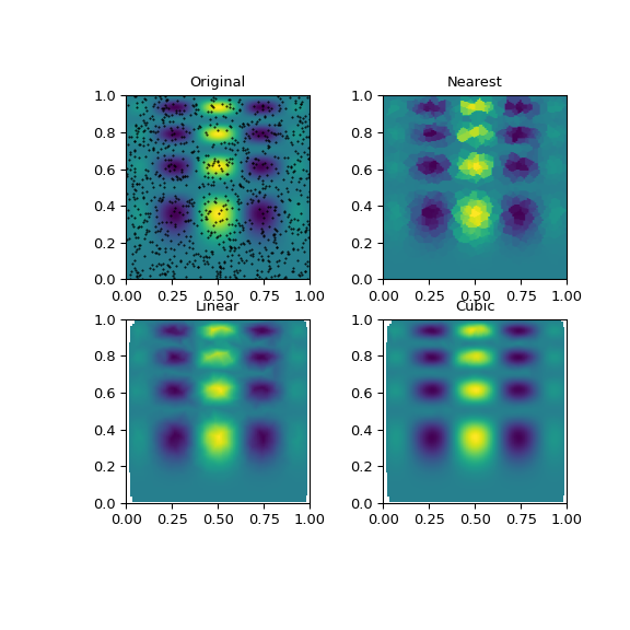
這可以使用 griddata 完成 – 下面,我們將嘗試所有內插方法
>>> from scipy.interpolate import griddata
>>> grid_z0 = griddata(points, values, (grid_x, grid_y), method='nearest')
>>> grid_z1 = griddata(points, values, (grid_x, grid_y), method='linear')
>>> grid_z2 = griddata(points, values, (grid_x, grid_y), method='cubic')
可以看出,所有方法都在某種程度上重現了精確的結果,但對於這個平滑函數,分段立方內插器給出了最佳結果(黑點顯示正在內插的資料)
>>> import matplotlib.pyplot as plt
>>> plt.subplot(221)
>>> plt.imshow(func(grid_x, grid_y).T, extent=(0, 1, 0, 1), origin='lower')
>>> plt.plot(points[:, 0], points[:, 1], 'k.', ms=1)   # data
>>> plt.title('Original')
>>> plt.subplot(222)
>>> plt.imshow(grid_z0.T, extent=(0, 1, 0, 1), origin='lower')
>>> plt.title('Nearest')
>>> plt.subplot(223)
>>> plt.imshow(grid_z1.T, extent=(0, 1, 0, 1), origin='lower')
>>> plt.title('Linear')
>>> plt.subplot(224)
>>> plt.imshow(grid_z2.T, extent=(0, 1, 0, 1), origin='lower')
>>> plt.title('Cubic')
>>> plt.gcf().set_size_inches(6, 6)
>>> plt.show()
對於每種內插方法,此函數都會委派給相應的類別物件 — 這些類別也可以直接使用 — NearestNDInterpolator、LinearNDInterpolator 和 CloughTocher2DInterpolator 用於 2D 中的分段立方內插。
所有這些內插方法都依賴於使用 QHull 函式庫(封裝在 scipy.spatial 中)對資料進行三角剖分。
注意
griddata 是基於三角剖分的,因此適用於非結構化、散佈的資料。如果您的資料位於完整網格上,則 griddata 函數(儘管其名稱如此)並不是正確的工具。請改用 RegularGridInterpolator。
注意
如果輸入資料的輸入維度具有不可比較的單位,並且相差許多數量級,則內插器可能會出現數值假影。考慮在內插之前重新調整資料的比例,或使用 rescale=True 關鍵字引數給 griddata。
使用徑向基底函數進行平滑/內插#
徑向基底函數可用於平滑/內插 N 維中的散佈資料,但對於觀察資料範圍之外的外插應謹慎使用。
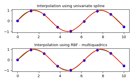
1-D 範例#
此範例比較了 RBFInterpolator 和 UnivariateSpline 類別在 scipy.interpolate 模組中的用法。
>>> import numpy as np
>>> from scipy.interpolate import RBFInterpolator, InterpolatedUnivariateSpline
>>> import matplotlib.pyplot as plt
>>> # setup data
>>> x = np.linspace(0, 10, 9).reshape(-1, 1)
>>> y = np.sin(x)
>>> xi = np.linspace(0, 10, 101).reshape(-1, 1)
>>> # use fitpack2 method
>>> ius = InterpolatedUnivariateSpline(x, y)
>>> yi = ius(xi)
>>> fix, (ax1, ax2) = plt.subplots(2, 1)
>>> ax1.plot(x, y, 'bo')
>>> ax1.plot(xi, yi, 'g')
>>> ax1.plot(xi, np.sin(xi), 'r')
>>> ax1.set_title('Interpolation using univariate spline')
>>> # use RBF method
>>> rbf = RBFInterpolator(x, y)
>>> fi = rbf(xi)
>>> ax2.plot(x, y, 'bo')
>>> ax2.plot(xi, fi, 'g')
>>> ax2.plot(xi, np.sin(xi), 'r')
>>> ax2.set_title('Interpolation using RBF - multiquadrics')
>>> plt.tight_layout()
>>> plt.show()
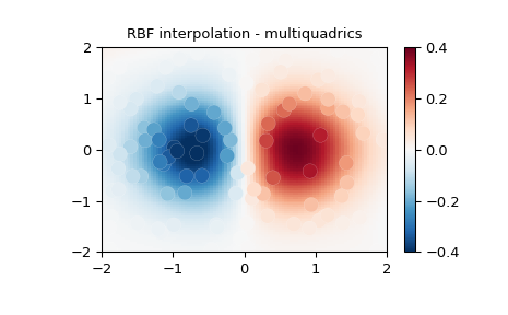
2-D 範例#
此範例示範如何內插散佈的 2 維資料
>>> import numpy as np
>>> from scipy.interpolate import RBFInterpolator
>>> import matplotlib.pyplot as plt
>>> # 2-d tests - setup scattered data
>>> rng = np.random.default_rng()
>>> xy = rng.random((100, 2))*4.0-2.0
>>> z = xy[:, 0]*np.exp(-xy[:, 0]**2-xy[:, 1]**2)
>>> edges = np.linspace(-2.0, 2.0, 101)
>>> centers = edges[:-1] + np.diff(edges[:2])[0] / 2.
>>> x_i, y_i = np.meshgrid(centers, centers)
>>> x_i = x_i.reshape(-1, 1)
>>> y_i = y_i.reshape(-1, 1)
>>> xy_i = np.concatenate([x_i, y_i], axis=1)
>>> # use RBF
>>> rbf = RBFInterpolator(xy, z, epsilon=2)
>>> z_i = rbf(xy_i)
>>> # plot the result
>>> fig, ax = plt.subplots()
>>> X_edges, Y_edges = np.meshgrid(edges, edges)
>>> lims = dict(cmap='RdBu_r', vmin=-0.4, vmax=0.4)
>>> mapping = ax.pcolormesh(
...     X_edges, Y_edges, z_i.reshape(100, 100),
...     shading='flat', **lims
... )
>>> ax.scatter(xy[:, 0], xy[:, 1], 100, z, edgecolor='w', lw=0.1, **lims)
>>> ax.set(
...     title='RBF interpolation - multiquadrics',
...     xlim=(-2, 2),
...     ylim=(-2, 2),
... )
>>> fig.colorbar(mapping)