內插過渡指南

本頁包含三組示範

• 用於舊版錯誤相容 scipy.interpolate.interp2d 替代方案的底層 FITPACK 替代方案；

• 新程式碼中建議使用的 scipy.interpolate.interp2d 替代方案；

• 以及基於 2D FITPACK 的線性內插的失敗模式示範和建議的替代方案。

1. 如何轉換為不使用 interp2d

interp2d 會在 2D 正規網格上的內插和 2D 散佈資料的內插之間靜默切換。此切換基於（展平的）x、y 和 z 陣列的長度。簡而言之，對於正規網格使用 scipy.interpolate.RectBivariateSpline；對於散佈內插，請使用 bisprep/bisplev 組合。下面我們給出逐點轉換的範例，這應能完全保留 interp2d 的結果。

1.1 interp2d 在正規網格上

我們從（稍微修改過的）文件字串範例開始。

>>> import numpy as np
>>> import matplotlib.pyplot as plt
>>> from scipy.interpolate import interp2d, RectBivariateSpline

>>> x = np.arange(-5.01, 5.01, 0.25)
>>> y = np.arange(-5.01, 7.51, 0.25)
>>> xx, yy = np.meshgrid(x, y)
>>> z = np.sin(xx**2 + 2.*yy**2)
>>> f = interp2d(x, y, z, kind='cubic')

這是「正規網格」程式碼路徑，因為

>>> z.size == len(x) * len(y)
True

另外，請注意 x.size != y.size

>>> x.size, y.size
(41, 51)

現在，讓我們建立一個方便的函式來建構內插器並繪製它。

>>> def plot(f, xnew, ynew):
...    fig, (ax1, ax2) = plt.subplots(1, 2, figsize=(8, 4))
...    znew = f(xnew, ynew)
...    ax1.plot(x, z[0, :], 'ro-', xnew, znew[0, :], 'b-')
...    im = ax2.imshow(znew)
...    plt.colorbar(im, ax=ax2)
...    plt.show()
...    return znew
...
>>> xnew = np.arange(-5.01, 5.01, 1e-2)
>>> ynew = np.arange(-5.01, 7.51, 1e-2)
>>> znew_i = plot(f, xnew, ynew)

替代方案：使用 RectBivariateSpline，結果相同

請注意轉置：首先，在建構函式中，其次，您需要轉置評估結果。這是為了撤銷 interp2d 所做的轉置。

>>> r = RectBivariateSpline(x, y, z.T)
>>> rt = lambda xnew, ynew: r(xnew, ynew).T
>>> znew_r = plot(rt, xnew, ynew)

>>> from numpy.testing import assert_allclose
>>> assert_allclose(znew_i, znew_r, atol=1e-14)

內插階數：線性、立方等

interp2d 預設為 kind="linear"，即在 x- 和 y- 兩個方向上都是線性的。RectBivariateSpline 另一方面，預設為立方內插，kx=3, ky=3。

這是完全等效的

interp2d	RectBivariateSpline
無 kwargs	kx = 1, ky = 1
kind=’linear’	kx = 1, ky = 1
kind=’cubic’	kx = 3, ky = 3

1.2. interp2d 具有點的完整座標（散佈內插）

在這裡，我們展平前一個練習中的網格，以說明此功能。

>>> xxr = xx.ravel()
>>> yyr = yy.ravel()
>>> zzr = z.ravel()
>>> f = interp2d(xxr, yyr, zzr, kind='cubic')

請注意，這是「非正規網格」程式碼路徑，適用於散佈資料，其中 len(x) == len(y) == len(z)。

>>> len(xxr) == len(yyr) == len(zzr)
True

>>> xnew = np.arange(-5.01, 5.01, 1e-2)
>>> ynew = np.arange(-5.01, 7.51, 1e-2)
>>> znew_i = plot(f, xnew, ynew)

替代方案：直接使用 scipy.interpolate.bisplrep / scipy.interpolate.bisplev

>>> from scipy.interpolate import bisplrep, bisplev
>>> tck = bisplrep(xxr, yyr, zzr, kx=3, ky=3, s=0)
# convenience: make up a callable from bisplev
>>> ff = lambda xnew, ynew: bisplev(xnew, ynew, tck).T   # Note the transpose, to mimic what interp2d does
>>> znew_b = plot(ff, xnew, ynew)

>>> assert_allclose(znew_i, znew_b, atol=1e-15)

內插階數：線性、立方等

interp2d 預設為 kind="linear"，即在 x- 和 y- 兩個方向上都是線性的。bisplrep 另一方面，預設為立方內插，kx=3, ky=3。

這是完全等效的

interp2d	bisplrep
無 kwargs	kx = 1, ky = 1
kind=’linear’	kx = 1, ky = 1
kind=’cubic’	kx = 3, ky = 3

2. interp2d 的替代方案：正規網格

對於新程式碼，建議的替代方案是 RegularGridInterpolator。它是一個獨立的實作，不是基於 FITPACK。支援最近鄰、線性內插和奇數階張量積樣條。

樣條節點保證與資料點重合。

請注意，在這裡

1. 元組引數是 (x, y)

2. z 陣列需要轉置

3. 關鍵字名稱是 *method*，而不是 *kind*

4. bounds_error 引數預設為 True。

>>> from scipy.interpolate import RegularGridInterpolator as RGI
>>> r = RGI((x, y), z.T, method='linear', bounds_error=False)

評估：建立 2D 網格。使用 indexing=’ij’ 和 sparse=True 以節省一些記憶體

>>> xxnew, yynew = np.meshgrid(xnew, ynew, indexing='ij', sparse=True)

評估，請注意元組引數

>>> znew_reggrid = r((xxnew, yynew))

>>> fig, (ax1, ax2) = plt.subplots(1, 2, figsize=(8, 4))
# Again, note the transpose to undo the `interp2d` convention
>>> znew_reggrid_t = znew_reggrid.T
>>> ax1.plot(x, z[0, :], 'ro-', xnew, znew_reggrid_t[0, :], 'b-')
>>> im = ax2.imshow(znew_reggrid_t)
>>> plt.colorbar(im, ax=ax2)

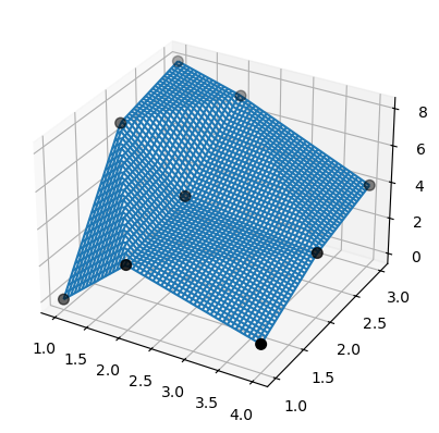
3. 散佈 2D 線性內插：偏好使用 LinearNDInterpolator 而不是 SmoothBivariateSpline 或 bisplrep

對於 2D 散佈線性內插，SmoothBivariateSpline 和 biplrep 都可能發出警告，或無法內插資料，或產生節點遠離資料點的樣條。相反地，偏好使用 LinearNDInterpolator，它基於透過 QHull 三角化資料。

# TestSmoothBivariateSpline::test_integral
>>> from scipy.interpolate import SmoothBivariateSpline, LinearNDInterpolator
>>> x = np.array([1,1,1,2,2,2,4,4,4])
>>> y = np.array([1,2,3,1,2,3,1,2,3])
>>> z = np.array([0,7,8,3,4,7,1,3,4])

現在，使用基於 Qhull 的資料三角化上的線性內插

>>> xy = np.c_[x, y]   # or just list(zip(x, y))
>>> lut2 = LinearNDInterpolator(xy, z)
>>> X = np.linspace(min(x), max(x))
>>> Y = np.linspace(min(y), max(y))
>>> X, Y = np.meshgrid(X, Y)

結果很容易理解和解釋

>>> fig = plt.figure()
>>> ax = fig.add_subplot(projection='3d')
>>> ax.plot_wireframe(X, Y, lut2(X, Y))
>>> ax.scatter(x, y, z,  'o', color='k', s=48)

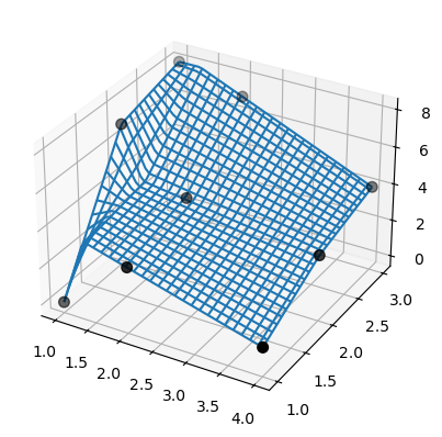
請注意，bisplrep 做的事情不同！它可能會將樣條節點放置在資料之外。

為了說明，請考慮與前一個範例相同的資料

>>> tck = bisplrep(x, y, z, kx=1, ky=1, s=0)
>>> fig = plt.figure()
>>> ax = fig.add_subplot(projection='3d')
>>> xx = np.linspace(min(x), max(x))
>>> yy = np.linspace(min(y), max(y))
>>> X, Y = np.meshgrid(xx, yy)
>>> Z = bisplev(xx, yy, tck)
>>> Z = Z.reshape(*X.shape).T
>>> ax.plot_wireframe(X, Y, Z, rstride=2, cstride=2)
>>> ax.scatter(x, y, z,  'o', color='k', s=48)

此外，SmoothBivariateSpline 無法內插資料。再次，使用與前一個範例相同的資料。

>>> lut = SmoothBivariateSpline(x, y, z, kx=1, ky=1, s=0)
>>> fig = plt.figure()
>>> ax = fig.add_subplot(projection='3d')
>>> xx = np.linspace(min(x), max(x))
>>> yy = np.linspace(min(y), max(y))
>>> X, Y = np.meshgrid(xx, yy)
>>> ax.plot_wireframe(X, Y, lut(xx, yy).T, rstride=4, cstride=4)
>>> ax.scatter(x, y, z,  'o', color='k', s=48)

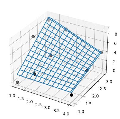
請注意，SmoothBivariateSpline 和 bisplrep 的結果都有瑕疵，這與 LinearNDInterpolator 的結果不同。此處說明的問題是針對線性內插回報的，但是 FITPACK 節點選擇機制不保證可以避免更高階（例如立方）樣條曲面的這些問題。