1-D 插值

分段線性插值

如果您只需要線性（又稱折線）插值，可以使用 numpy.interp 常式。它接受兩個資料陣列進行插值，x 和 y，以及第三個陣列 xnew，用於評估插值的點

>>> import numpy as np
>>> x = np.linspace(0, 10, num=11)
>>> y = np.cos(-x**2 / 9.0)

建構插值

>>> xnew = np.linspace(0, 10, num=1001)
>>> ynew = np.interp(xnew, x, y)

並繪製它

>>> import matplotlib.pyplot as plt
>>> plt.plot(xnew, ynew, '-', label='linear interp')
>>> plt.plot(x, y, 'o', label='data')
>>> plt.legend(loc='best')
>>> plt.show()

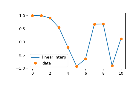
numpy.interp 的一個限制是它不允許控制外插。有關提供此類功能的替代常式，請參閱 使用 B 樣條插值區段。

三次樣條

當然，分段線性插值在資料點處會產生角點，線性片段在此處連接。為了產生更平滑的曲線，您可以使用三次樣條，其中插值曲線由具有匹配的一階和二階導數的三次片段組成。在程式碼中，這些物件透過 CubicSpline 類別實例表示。實例是使用資料的 x 和 y 陣列建構的，然後可以使用目標 xnew 值進行評估

>>> from scipy.interpolate import CubicSpline
>>> spl = CubicSpline([1, 2, 3, 4, 5, 6], [1, 4, 8, 16, 25, 36])
>>> spl(2.5)
5.57

CubicSpline 物件的 __call__ 方法接受純量值和陣列。它還接受第二個引數 nu，以評估 nu 階導數。例如，我們繪製樣條的導數

>>> from scipy.interpolate import CubicSpline
>>> x = np.linspace(0, 10, num=11)
>>> y = np.cos(-x**2 / 9.)
>>> spl = CubicSpline(x, y)

>>> import matplotlib.pyplot as plt
>>> fig, ax = plt.subplots(4, 1, figsize=(5, 7))
>>> xnew = np.linspace(0, 10, num=1001)
>>> ax[0].plot(xnew, spl(xnew))
>>> ax[0].plot(x, y, 'o', label='data')
>>> ax[1].plot(xnew, spl(xnew, nu=1), '--', label='1st derivative')
>>> ax[2].plot(xnew, spl(xnew, nu=2), '--', label='2nd derivative')
>>> ax[3].plot(xnew, spl(xnew, nu=3), '--', label='3rd derivative')
>>> for j in range(4):
...     ax[j].legend(loc='best')
>>> plt.tight_layout()
>>> plt.show()

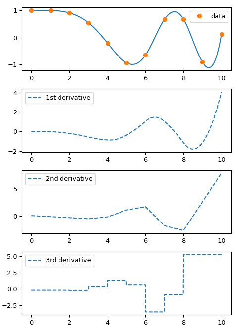
請注意，根據建構，一階和二階導數是連續的，而三階導數在資料點處跳躍。

單調插值器

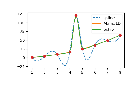
根據建構，三次樣條是兩次連續可微分的。這可能會導致樣條函數在資料點之間振盪和「過衝」。在這些情況下，另一種選擇是使用所謂的單調三次插值器：這些插值器建構成僅一次連續可微分，並嘗試保留資料暗示的局部形狀。scipy.interpolate 提供了兩種此類物件：PchipInterpolator 和 Akima1DInterpolator 。為了說明，我們考慮具有離群值的資料

>>> from scipy.interpolate import CubicSpline, PchipInterpolator, Akima1DInterpolator
>>> x = np.array([1., 2., 3., 4., 4.5, 5., 6., 7., 8])
>>> y = x**2
>>> y[4] += 101

>>> import matplotlib.pyplot as plt
>>> xx = np.linspace(1, 8, 51)
>>> plt.plot(xx, CubicSpline(x, y)(xx), '--', label='spline')
>>> plt.plot(xx, Akima1DInterpolator(x, y)(xx), '-', label='Akima1D')
>>> plt.plot(xx, PchipInterpolator(x, y)(xx), '-', label='pchip')
>>> plt.plot(x, y, 'o')
>>> plt.legend()
>>> plt.show()

使用 B 樣條插值

B 樣條形成了分段多項式的替代（如果形式上等效）表示法。此基底通常比冪基底在計算上更穩定，並且適用於包括插值、迴歸和曲線表示在內的各種應用。詳細資訊在 分段多項式區段 中給出，在這裡我們透過建構正弦函數的插值來說明它們的用法

>>> x = np.linspace(0, 3/2, 7)
>>> y = np.sin(np.pi*x)

為了建構給定資料陣列 x 和 y 的插值物件，我們使用 make_interp_spline 函數

>>> from scipy.interpolate import make_interp_spline
>>> bspl = make_interp_spline(x, y, k=3)

此函數傳回一個物件，該物件具有與 CubicSpline 物件類似的介面。特別是，它可以在資料點處進行評估和微分

>>> der = bspl.derivative()      # a BSpline representing the derivative
>>> import matplotlib.pyplot as plt
>>> xx = np.linspace(0, 3/2, 51)
>>> plt.plot(xx, bspl(xx), '--', label=r'$\sin(\pi x)$ approx')
>>> plt.plot(x, y, 'o', label='data')
>>> plt.plot(xx, der(xx)/np.pi, '--', label=r'$d \sin(\pi x)/dx / \pi$ approx')
>>> plt.legend()
>>> plt.show()

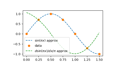
請注意，透過在 make_interp_spline 呼叫中指定 k=3，我們請求了三次樣條（這是預設值，因此可以省略 k=3）；三次的導數是二次

>>> bspl.k, der.k
(3, 2)

預設情況下，make_interp_spline(x, y) 的結果等效於 CubicSpline(x, y)。不同之處在於前者允許幾種可選功能：它可以建構各種次數的樣條（透過可選引數 k）和預定義的節點（透過可選引數 t）。

樣條插值的邊界條件可以透過 make_interp_spline 函數和 CubicSpline 建構函式的 bc_type 引數來控制。預設情況下，兩者都使用「not-a-knot」邊界條件。

非三次樣條

make_interp_spline 的一種用途是建構具有線性外插的線性插值器，因為 make_interp_spline 預設會進行外插。考慮

>>> from scipy.interpolate import make_interp_spline
>>> x = np.linspace(0, 5, 11)
>>> y = 2*x
>>> spl = make_interp_spline(x, y, k=1)  # k=1: linear
>>> spl([-1, 6])
[-2., 12.]
>>> np.interp([-1, 6], x, y)
[0., 10.]

有關更多詳細資訊和討論，請參閱 外插區段。

參數樣條曲線

到目前為止，我們考慮了樣條函數，其中資料 y 預期顯式地依賴於自變數 x——因此插值函數滿足 \(f(x_j) = y_j\)。樣條曲線將 x 和 y 陣列視為平面上點 \(\mathbf{p}_j\) 的座標，以及通過這些點的插值曲線由一些額外的參數（通常稱為 u）參數化。請注意，此建構很容易推廣到更高維度，其中 \(\mathbf{p}_j\) 是 N 維空間中的點。

可以使用插值函數處理多維資料陣列這一事實輕鬆建構樣條曲線。對應於資料點的參數 u 的值需要由使用者單獨提供。

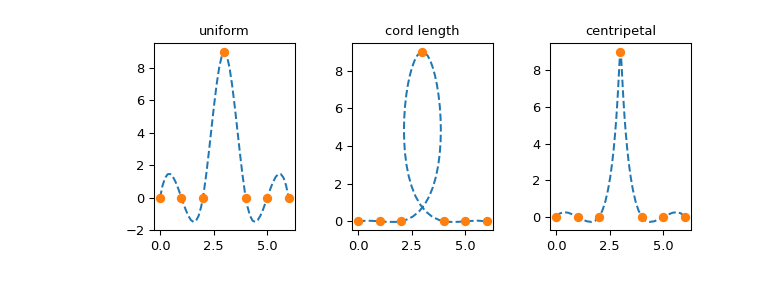
參數化的選擇取決於問題，不同的參數化可能會產生截然不同的曲線。作為一個範例，我們考慮（有些困難的）資料集的三種參數化，我們從參考文獻 [1] 的第 6 章中取得，該文獻列在 BSpline 文件字串中

>>> x = [0, 1, 2, 3, 4, 5, 6]
>>> y = [0, 0, 0, 9, 0, 0, 0]
>>> p = np.stack((x, y))
>>> p
array([[0, 1, 2, 3, 4, 5, 6],
       [0, 0, 0, 9, 0, 0, 0]])

我們將 p 陣列的元素作為平面上七個點的座標，其中 p[:, j] 給出點 \(\mathbf{p}_j\) 的座標。

首先，考慮均勻參數化，\(u_j = j\)

>>> u_unif = x

其次，我們考慮所謂的弦長參數化，它只不過是連接資料點的直線段的累積長度

\[u_j = u_{j-1} + |\mathbf{p}_j - \mathbf{p}_{j-1}|\]

對於 \(j=1, 2, \dots\) 和 \(u_0 = 0\)。這裡 \(| \cdots |\) 是平面上連續點 \(p_j\) 之間的長度。

>>> dp = p[:, 1:] - p[:, :-1]      # 2-vector distances between points
>>> l = (dp**2).sum(axis=0)        # squares of lengths of 2-vectors between points
>>> u_cord = np.sqrt(l).cumsum()   # cumulative sums of 2-norms
>>> u_cord = np.r_[0, u_cord]      # the first point is parameterized at zero

最後，我們考慮有時稱為向心參數化的方法：\(u_j = u_{j-1} + |\mathbf{p}_j - \mathbf{p}_{j-1}|^{1/2}\)。由於額外的平方根，連續值 \(u_j - u_{j-1}\) 之間的差異將小於弦長參數化的差異

>>> u_c = np.r_[0, np.cumsum((dp**2).sum(axis=0)**0.25)]

現在繪製結果曲線

>>> from scipy.interpolate import make_interp_spline
>>> import matplotlib.pyplot as plt
>>> fig, ax = plt.subplots(1, 3, figsize=(8, 3))
>>> parametrizations = ['uniform', 'cord length', 'centripetal']
>>>
>>> for j, u in enumerate([u_unif, u_cord, u_c]):
...    spl = make_interp_spline(u, p, axis=1)    # note p is a 2D array
...
...    uu = np.linspace(u[0], u[-1], 51)
...    xx, yy = spl(uu)
...
...    ax[j].plot(xx, yy, '--')
...    ax[j].plot(p[0, :], p[1, :], 'o')
...    ax[j].set_title(parametrizations[j])
>>> plt.show()

1-D 插值的傳統介面 (interp1d)

注意

interp1d 被認為是傳統 API，不建議在新程式碼中使用。考慮使用更具體的插值器來代替。

interp1d 類別在 scipy.interpolate 中是一種方便的方法，用於建立基於固定資料點的函數，該函數可以使用線性插值在給定資料定義的域內的任何位置進行評估。此類別的實例是透過傳遞包含資料的 1-D 向量來建立的。此類別的實例定義了一個 __call__ 方法，因此可以像一個函數一樣處理，該函數在已知資料值之間進行插值以獲得未知值。邊界處的行為可以在實例化時指定。以下範例示範了其用法，用於線性和三次樣條插值

>>> from scipy.interpolate import interp1d

>>> x = np.linspace(0, 10, num=11, endpoint=True)
>>> y = np.cos(-x**2/9.0)
>>> f = interp1d(x, y)
>>> f2 = interp1d(x, y, kind='cubic')

>>> xnew = np.linspace(0, 10, num=41, endpoint=True)
>>> import matplotlib.pyplot as plt
>>> plt.plot(x, y, 'o', xnew, f(xnew), '-', xnew, f2(xnew), '--')
>>> plt.legend(['data', 'linear', 'cubic'], loc='best')
>>> plt.show()

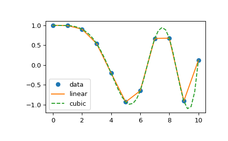
「cubic」種類的 interp1d 等效於 make_interp_spline，而「linear」種類等效於 numpy.interp，同時也允許 N 維 y 陣列。

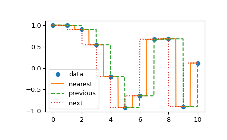
interp1d 中的另一組插值是 nearest、previous 和 next，它們分別傳回沿 x 軸最近、之前或之後的點。最近和下一個可以被認為是因果插值濾波器的特例。以下範例示範了它們的用法，使用與前一個範例相同的資料

>>> from scipy.interpolate import interp1d

>>> x = np.linspace(0, 10, num=11, endpoint=True)
>>> y = np.cos(-x**2/9.0)
>>> f1 = interp1d(x, y, kind='nearest')
>>> f2 = interp1d(x, y, kind='previous')
>>> f3 = interp1d(x, y, kind='next')

>>> xnew = np.linspace(0, 10, num=1001, endpoint=True)
>>> import matplotlib.pyplot as plt
>>> plt.plot(x, y, 'o')
>>> plt.plot(xnew, f1(xnew), '-', xnew, f2(xnew), '--', xnew, f3(xnew), ':')
>>> plt.legend(['data', 'nearest', 'previous', 'next'], loc='best')
>>> plt.show()

interp1d 模式的建議替代方案

如前所述，interp1d 類別是傳統的：我們沒有移除它的計劃；我們將繼續支援其現有的用法；但是我們相信有更好的替代方案，我們建議在新程式碼中使用。

在這裡，我們列出了具體的建議，具體取決於插值 kind。

線性插值， kind="linear"

預設建議是使用 numpy.interp 函數。或者，您可以使用線性樣條，make_interp_spline(x, y, k=1)，請參閱 本節的討論。

樣條插值器， kind="quadratic" 或 "cubic"

在底層，interp1d 委派給 make_interp_spline，因此我們建議直接使用後者。

分段常數模式， kind="nearest", "previous", "next"

首先，我們注意到 interp1d(x, y, kind='previous') 等效於 make_interp_spline(x, y, k=0)。

然而，更一般地，所有這些分段常數插值模式都基於 numpy.searchsorted。例如，"nearest" 模式只不過是

>>> x = np.arange(8)
>>> y = x**2
>>> x_new = np.linspace(0, 7, 101)    # input points
>>> x_bds = x[:-1] / 2.0 + x[1:] / 2.0   # halfway points
>>> idx = np.searchsorted(x_bds, x_new, side='left')
>>> idx = np.clip(idx, 0, len(x) - 1)  # clip the indices so that they are within the range of x indices.
>>> import matplotlib.pyplot as plt
>>> plt.plot(x, y, 'o')
>>> plt.plot(x_new, y[idx], '--')
>>> plt.show()

其他變體類似，有關詳細資訊，請參閱 interp1d 原始碼。

遺失資料

我們注意到 scipy.interpolate 不支援使用遺失資料進行插值。表示遺失資料的兩種常用方法是使用 numpy.ma 程式庫的遮罩陣列，以及將遺失值編碼為非數字 NaN。

這兩種方法在 scipy.interpolate 中都不直接支援。個別常式可能提供部分支援和/或解決方案，但總體而言，該程式庫堅定地遵守 IEEE 754 語意，其中 NaN 表示非數字，即非法數學運算的結果（想想除以零），而不是遺失。