scipy.stats.invwishart

scipy.stats.invwishart = <scipy.stats._multivariate.invwishart_gen object>

反 Wishart 隨機變數。

df 關鍵字指定自由度。scale 關鍵字指定尺度矩陣，其必須為對稱且正定的。在此上下文中，尺度矩陣通常以多變量常態共變異數矩陣來解釋。

參數:

dfint

自由度，必須大於或等於尺度矩陣的維度

scalearray_like

分布的對稱正定尺度矩陣

seed{None, int, np.random.RandomState, np.random.Generator}, 選用

用於繪製隨機變量。如果 seed 為 None，則使用 RandomState 單例。如果 seed 是整數，則使用新的 RandomState 實例，並以 seed 作為種子。如果 seed 已經是 RandomState 或 Generator 實例，則使用該物件。預設為 None。

引發:

scipy.linalg.LinAlgError

如果尺度矩陣 scale 不是正定的。

另請參閱

wishart

註解

尺度矩陣 scale 必須是對稱正定矩陣。不支援奇異矩陣，包括對稱正半定情況。不檢查對稱性；僅使用下三角部分。

反 Wishart 分布通常表示為

\[W_p^{-1}(\nu, \Psi)\]

其中 \(\nu\) 是自由度，而 \(\Psi\) 是 \(p \times p\) 尺度矩陣。

對於 invwishart 的機率密度函數，其支援範圍為正定矩陣 \(S\)；如果 \(S \sim W^{-1}_p(\nu, \Sigma)\)，則其 PDF 由下式給出

\[f(S) = \frac{|\Sigma|^\frac{\nu}{2}}{2^{ \frac{\nu p}{2} } |S|^{\frac{\nu + p + 1}{2}} \Gamma_p \left(\frac{\nu}{2} \right)} \exp\left( -tr(\Sigma S^{-1}) / 2 \right)\]

如果 \(S \sim W_p^{-1}(\nu, \Psi)\) (反 Wishart)，則 \(S^{-1} \sim W_p(\nu, \Psi^{-1})\) (Wishart)。

如果尺度矩陣是 1 維且等於 1，則反 Wishart 分布 \(W_1(\nu, 1)\) 會塌縮為反 Gamma 分布，其參數 shape = \(\frac{\nu}{2}\) 且 scale = \(\frac{1}{2}\)。

此處未使用 [2] 中描述的隨機生成 Wishart 矩陣並進行反轉，而是使用 [4] 中的演算法直接生成隨機反 Wishart 矩陣，而無需反轉。

在 0.16.0 版本中新增。

參考文獻

[1]

M.L. Eaton, “Multivariate Statistics: A Vector Space Approach”, Wiley, 1983.

[2]

M.C. Jones, “Generating Inverse Wishart Matrices”, Communications in Statistics - Simulation and Computation, vol. 14.2, pp.511-514, 1985.

[3]

Gupta, M. and Srivastava, S. “Parametric Bayesian Estimation of Differential Entropy and Relative Entropy”. Entropy 12, 818 - 843. 2010.

[4]

S.D. Axen, “Efficiently generating inverse-Wishart matrices and their Cholesky factors”, arXiv:2310.15884v1. 2023.

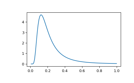
範例

在您的瀏覽器中試試看！

>>> import numpy as np
>>> import matplotlib.pyplot as plt
>>> from scipy.stats import invwishart, invgamma
>>> x = np.linspace(0.01, 1, 100)
>>> iw = invwishart.pdf(x, df=6, scale=1)
>>> iw[:3]
array([  1.20546865e-15,   5.42497807e-06,   4.45813929e-03])
>>> ig = invgamma.pdf(x, 6/2., scale=1./2)
>>> ig[:3]
array([  1.20546865e-15,   5.42497807e-06,   4.45813929e-03])
>>> plt.plot(x, iw)
>>> plt.show()

輸入分位數可以是任何形狀的陣列，只要最後一個軸標記組件即可。

或者，可以呼叫物件（作為函數）以固定自由度和尺度參數，傳回「凍結」的反 Wishart 隨機變數

>>> rv = invwishart(df=1, scale=1)
>>> # Frozen object with the same methods but holding the given
>>> # degrees of freedom and scale fixed.

返回在新分頁中開啟

方法

pdf(x, df, scale)	機率密度函數。
logpdf(x, df, scale)	機率密度函數的對數。
rvs(df, scale, size=1, random_state=None)	從反 Wishart 分布中繪製隨機樣本。
entropy(df, scale)	分布的微分熵。