scipy.stats.

cumfreq#

scipy.stats.cumfreq(a, numbins=10, defaultreallimits=None, weights=None)[source]#

返回累積頻率直方圖，使用 histogram 函數。

累積直方圖是一種映射，用於計算直到指定 bin 的所有 bin 中累積的觀測值數量。

參數:

aarray_like: 輸入陣列。
numbinsint，可選: 用於直方圖的 bin 數量。預設值為 10。
defaultreallimitstuple (lower, upper)，可選: 直方圖範圍的下限和上限值。如果未給定值，則使用略大於 a 中值範圍的範圍。具體而言，(a.min() - s, a.max() + s)，其中 s = (1/2)(a.max() - a.min()) / (numbins - 1)。
weightsarray_like，可選: a 中每個值的權重。預設值為 None，這會給每個值 1.0 的權重。

返回:

cumcountndarray: 累積頻率的 bin 值。
lowerlimitfloat: 下限實數
binsizefloat: 每個 bin 的寬度。
extrapointsint: 額外點。

範例

>>> import numpy as np
>>> import matplotlib.pyplot as plt
>>> from scipy import stats
>>> rng = np.random.default_rng()
>>> x = [1, 4, 2, 1, 3, 1]
>>> res = stats.cumfreq(x, numbins=4, defaultreallimits=(1.5, 5))
>>> res.cumcount
array([ 1.,  2.,  3.,  3.])
>>> res.extrapoints
3

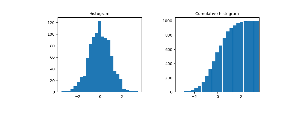
建立具有 1000 個隨機值的常態分佈

>>> samples = stats.norm.rvs(size=1000, random_state=rng)

計算累積頻率

>>> res = stats.cumfreq(samples, numbins=25)

計算 x 值的空間

>>> x = res.lowerlimit + np.linspace(0, res.binsize*res.cumcount.size,
...                                  res.cumcount.size)

繪製直方圖和累積直方圖

>>> fig = plt.figure(figsize=(10, 4))
>>> ax1 = fig.add_subplot(1, 2, 1)
>>> ax2 = fig.add_subplot(1, 2, 2)
>>> ax1.hist(samples, bins=25)
>>> ax1.set_title('Histogram')
>>> ax2.bar(x, res.cumcount, width=res.binsize)
>>> ax2.set_title('Cumulative histogram')
>>> ax2.set_xlim([x.min(), x.max()])

>>> plt.show()