scipy.stats.

binned_statistic

scipy.stats.binned_statistic(x, values, statistic='mean', bins=10, range=None)

為一或多組資料計算分箱統計量。

這是直方圖函數的推廣。直方圖將空間劃分為箱，並傳回每個箱中點的計數。此函數允許計算每個箱內的值（或值集）的總和、平均值、中位數或其他統計量。

參數:

x(N,) 類陣列

要分箱的值序列。

values(N,) 類陣列或 (N,) 類陣列的列表

將在其上計算統計量的資料。這必須與 x 的形狀相同，或是一組序列 - 每個序列都與 x 的形狀相同。如果 values 是一組序列，則將獨立計算每個序列的統計量。

statistic字串或可呼叫物件，選用

要計算的統計量（預設為 ‘mean’）。可用的統計量如下

• ‘mean’ : 計算每個箱內點的值的平均值。空箱將以 NaN 表示。

• ‘std’ : 計算每個箱內的標準差。這是隱式使用 ddof=0 計算的。

• ‘median’ : 計算每個箱內點的值的中位數。空箱將以 NaN 表示。

• ‘count’ : 計算每個箱內點的計數。這與未加權的直方圖相同。values 陣列未被參考。

• ‘sum’ : 計算每個箱內點的值的總和。這與加權直方圖相同。

• ‘min’ : 計算每個箱內點的值的最小值。空箱將以 NaN 表示。

• ‘max’ : 計算每個箱內點的值的最大值。空箱將以 NaN 表示。

• function : 使用者定義的函數，它接受一維值陣列，並輸出單一數值統計量。此函數將在每個箱中的值上呼叫。空箱將以 function([]) 表示，如果這傳回錯誤，則為 NaN。

bins整數或純量序列，選用

如果 bins 是整數，則它定義給定範圍內等寬箱的數量（預設為 10）。如果 bins 是一個序列，則它定義箱邊緣，包括最右邊的邊緣，允許非均勻的箱寬。x 中小於最低箱邊緣的值會被分配到箱號 0，超出最高箱的值會被分配到 bins[-1]。如果指定了箱邊緣，則箱的數量將為 (nx = len(bins)-1)。

range(float, float) 或 [(float, float)]，選用

箱的下限和上限範圍。如果未提供，範圍就只是 (x.min(), x.max())。範圍外的值將被忽略。

傳回值:

statistic陣列

每個箱中選定統計量的值。

bin_edges浮點數 dtype 的陣列

傳回箱邊緣 (length(statistic)+1)。

binnumber: 1-D ndarray of ints

箱的索引（對應於 bin_edges），x 的每個值都屬於這些箱。與 values 的長度相同。binnumber 為 i 表示對應值介於 (bin_edges[i-1], bin_edges[i]) 之間。

另請參閱

numpy.digitize, numpy.histogram, binned_statistic_2d, binned_statistic_dd

註解

除了最後一個（最右邊的）箱之外，所有箱都是半開區間。換句話說，如果 bins 是 [1, 2, 3, 4]，則第一個箱是 [1, 2)（包含 1，但不包含 2），第二個箱是 [2, 3)。然而，最後一個箱是 [3, 4]，它包含 4。

在版本 0.11.0 中新增。

範例

在您的瀏覽器中試試看！

>>> import numpy as np
>>> from scipy import stats
>>> import matplotlib.pyplot as plt

首先是一些基本範例

在給定樣本的範圍內建立兩個均勻間隔的箱，並將每個箱中對應的值加總

>>> values = [1.0, 1.0, 2.0, 1.5, 3.0]
>>> stats.binned_statistic([1, 1, 2, 5, 7], values, 'sum', bins=2)
BinnedStatisticResult(statistic=array([4. , 4.5]),
        bin_edges=array([1., 4., 7.]), binnumber=array([1, 1, 1, 2, 2]))

也可以傳遞多個值陣列。統計量是針對每個集合獨立計算的

>>> values = [[1.0, 1.0, 2.0, 1.5, 3.0], [2.0, 2.0, 4.0, 3.0, 6.0]]
>>> stats.binned_statistic([1, 1, 2, 5, 7], values, 'sum', bins=2)
BinnedStatisticResult(statistic=array([[4. , 4.5],
       [8. , 9. ]]), bin_edges=array([1., 4., 7.]),
       binnumber=array([1, 1, 1, 2, 2]))

>>> stats.binned_statistic([1, 2, 1, 2, 4], np.arange(5), statistic='mean',
...                        bins=3)
BinnedStatisticResult(statistic=array([1., 2., 4.]),
        bin_edges=array([1., 2., 3., 4.]),
        binnumber=array([1, 2, 1, 2, 3]))

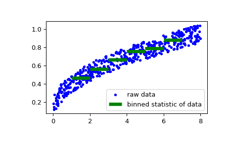
作為第二個範例，我們現在產生一些帆船速度的隨機資料，作為風速的函數，然後確定我們的船在特定風速下的速度有多快

>>> rng = np.random.default_rng()
>>> windspeed = 8 * rng.random(500)
>>> boatspeed = .3 * windspeed**.5 + .2 * rng.random(500)
>>> bin_means, bin_edges, binnumber = stats.binned_statistic(windspeed,
...                 boatspeed, statistic='median', bins=[1,2,3,4,5,6,7])
>>> plt.figure()
>>> plt.plot(windspeed, boatspeed, 'b.', label='raw data')
>>> plt.hlines(bin_means, bin_edges[:-1], bin_edges[1:], colors='g', lw=5,
...            label='binned statistic of data')
>>> plt.legend()

現在我們可以使用 binnumber 來選擇所有風速低於 1 的資料點

>>> low_boatspeed = boatspeed[binnumber == 0]

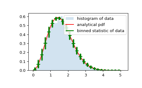
作為最後一個範例，我們將使用 bin_edges 和 binnumber 來繪製分佈圖，該分佈圖顯示每個箱的平均值和圍繞該平均值的分佈，以及常規直方圖和機率分佈函數

>>> x = np.linspace(0, 5, num=500)
>>> x_pdf = stats.maxwell.pdf(x)
>>> samples = stats.maxwell.rvs(size=10000)

>>> bin_means, bin_edges, binnumber = stats.binned_statistic(x, x_pdf,
...         statistic='mean', bins=25)
>>> bin_width = (bin_edges[1] - bin_edges[0])
>>> bin_centers = bin_edges[1:] - bin_width/2

>>> plt.figure()
>>> plt.hist(samples, bins=50, density=True, histtype='stepfilled',
...          alpha=0.2, label='histogram of data')
>>> plt.plot(x, x_pdf, 'r-', label='analytical pdf')
>>> plt.hlines(bin_means, bin_edges[:-1], bin_edges[1:], colors='g', lw=2,
...            label='binned statistic of data')
>>> plt.plot((binnumber - 0.5) * bin_width, x_pdf, 'g.', alpha=0.5)
>>> plt.legend(fontsize=10)
>>> plt.show()

返回在新分頁中開啟