scipy.stats.

bayes_mvs#

scipy.stats.bayes_mvs(data, alpha=0.9)[source]#

平均值、變異數和標準差的貝氏信賴區間。

參數:

dataarray_like（類陣列）: 輸入資料，如果是多維資料，它會被 bayes_mvs 展平成 1 維資料。需要 2 個或更多資料點。
alphafloat, optional（可選）: 返回的信賴區間包含真實參數的機率。

回傳:

mean_cntr, var_cntr, std_cntrtuple

三個結果分別是平均值、變異數和標準差。每個結果都是以下形式的元組

(center, (lower, upper))

其中 center 是給定資料下值的條件機率密度函數 (pdf) 的平均值，而 (lower, upper) 是一個信賴區間，以中位數為中心，包含機率為 alpha 的估計值。

另請參閱

mvsdist

註解

每個平均值、變異數和標準差估計值的元組都表示 (center, (lower, upper))，其中 center 是給定資料下值的條件機率密度函數 (pdf) 的平均值，而 (lower, upper) 是一個以中位數為中心的信賴區間，包含機率為 alpha 的估計值。

將資料轉換為 1 維，並假設所有資料都具有相同的平均值和變異數。變異數和標準差使用 Jeffrey 事前分佈。

相當於 tuple((x.mean(), x.interval(alpha)) for x in mvsdist(dat))

參考文獻

T.E. Oliphant, “A Bayesian perspective on estimating mean, variance, and standard-deviation from data”, https://scholarsarchive.byu.edu/facpub/278, 2006.

範例

首先，一個基本範例來示範輸出

>>> from scipy import stats
>>> data = [6, 9, 12, 7, 8, 8, 13]
>>> mean, var, std = stats.bayes_mvs(data)
>>> mean
Mean(statistic=9.0, minmax=(7.103650222612533, 10.896349777387467))
>>> var
Variance(statistic=10.0, minmax=(3.176724206, 24.45910382))
>>> std
Std_dev(statistic=2.9724954732045084,
        minmax=(1.7823367265645143, 4.945614605014631))

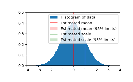
現在我們產生一些常態分佈的隨機資料，並取得這些估計值的平均值和標準差的 95% 信賴區間估計值

>>> n_samples = 100000
>>> data = stats.norm.rvs(size=n_samples)
>>> res_mean, res_var, res_std = stats.bayes_mvs(data, alpha=0.95)

>>> import matplotlib.pyplot as plt
>>> fig = plt.figure()
>>> ax = fig.add_subplot(111)
>>> ax.hist(data, bins=100, density=True, label='Histogram of data')
>>> ax.vlines(res_mean.statistic, 0, 0.5, colors='r', label='Estimated mean')
>>> ax.axvspan(res_mean.minmax[0],res_mean.minmax[1], facecolor='r',
...            alpha=0.2, label=r'Estimated mean (95% limits)')
>>> ax.vlines(res_std.statistic, 0, 0.5, colors='g', label='Estimated scale')
>>> ax.axvspan(res_std.minmax[0],res_std.minmax[1], facecolor='g', alpha=0.2,
...            label=r'Estimated scale (95% limits)')

>>> ax.legend(fontsize=10)
>>> ax.set_xlim([-4, 4])
>>> ax.set_ylim([0, 0.5])
>>> plt.show()

../../_images/scipy-stats-bayes_mvs-1.png