scipy.special.voigt_profile#

scipy.special.voigt_profile(x, sigma, gamma, out=None) = <ufunc 'voigt_profile'>#

Voigt 剖面。

Voigt 剖面是一個 1-D 常態分佈（標準差為 sigma）和 1-D 柯西分佈（半高寬為 gamma）的卷積。

如果 sigma = 0，則返回柯西分佈的 PDF。相反地，如果 gamma = 0，則返回常態分佈的 PDF。如果 sigma = gamma = 0，則當 x = 0 時返回值為 Inf，對於所有其他 x 則為 0。

參數:

xarray_like: 實數引數
sigmaarray_like: 常態分佈部分的標準差
gammaarray_like: 柯西分佈部分的半高寬
outndarray, optional: 函數值的可選輸出陣列

返回:

純量或 ndarray: 給定引數的 Voigt 剖面

參見

wofz: Faddeeva 函數

註解

它可以表示為 Faddeeva 函數的形式

\[V(x; \sigma, \gamma) = \frac{Re[w(z)]}{\sigma\sqrt{2\pi}},\]

\[z = \frac{x + i\gamma}{\sqrt{2}\sigma}\]

其中 \(w(z)\) 是 Faddeeva 函數。

參考文獻

[1]

https://en.wikipedia.org/wiki/Voigt_profile

範例

計算 sigma=1 和 gamma=1 時，點 2 的函數值。

>>> from scipy.special import voigt_profile
>>> import numpy as np
>>> import matplotlib.pyplot as plt
>>> voigt_profile(2, 1., 1.)
0.09071519942627544

通過為 x 提供 NumPy 陣列，計算多個點的函數值。

>>> values = np.array([-2., 0., 5])
>>> voigt_profile(values, 1., 1.)
array([0.0907152 , 0.20870928, 0.01388492])

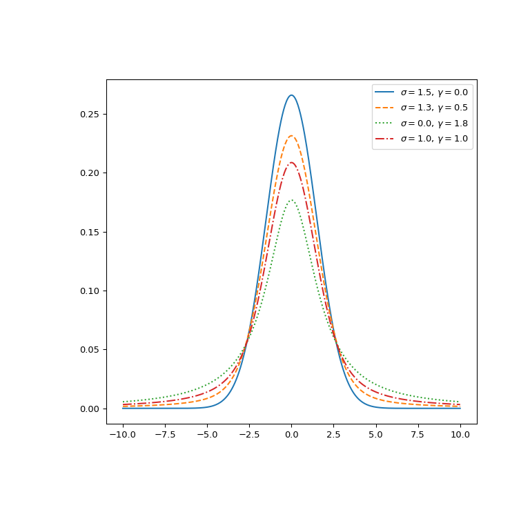
繪製不同參數集的函數圖。

>>> fig, ax = plt.subplots(figsize=(8, 8))
>>> x = np.linspace(-10, 10, 500)
>>> parameters_list = [(1.5, 0., "solid"), (1.3, 0.5, "dashed"),
...                    (0., 1.8, "dotted"), (1., 1., "dashdot")]
>>> for params in parameters_list:
...     sigma, gamma, linestyle = params
...     voigt = voigt_profile(x, sigma, gamma)
...     ax.plot(x, voigt, label=rf"$\sigma={sigma},\, \gamma={gamma}$",
...             ls=linestyle)
>>> ax.legend()
>>> plt.show()

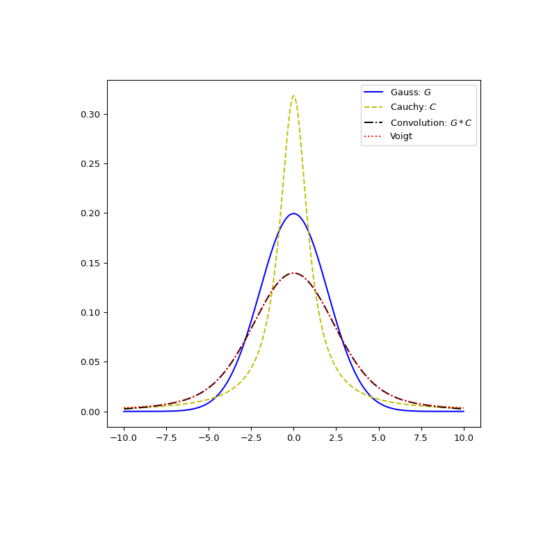
視覺化驗證 Voigt 剖面確實是由常態分佈和柯西分佈的卷積產生的。

>>> from scipy.signal import convolve
>>> x, dx = np.linspace(-10, 10, 500, retstep=True)
>>> def gaussian(x, sigma):
...     return np.exp(-0.5 * x**2/sigma**2)/(sigma * np.sqrt(2*np.pi))
>>> def cauchy(x, gamma):
...     return gamma/(np.pi * (np.square(x)+gamma**2))
>>> sigma = 2
>>> gamma = 1
>>> gauss_profile = gaussian(x, sigma)
>>> cauchy_profile = cauchy(x, gamma)
>>> convolved = dx * convolve(cauchy_profile, gauss_profile, mode="same")
>>> voigt = voigt_profile(x, sigma, gamma)
>>> fig, ax = plt.subplots(figsize=(8, 8))
>>> ax.plot(x, gauss_profile, label="Gauss: $G$", c='b')
>>> ax.plot(x, cauchy_profile, label="Cauchy: $C$", c='y', ls="dashed")
>>> xx = 0.5*(x[1:] + x[:-1])  # midpoints
>>> ax.plot(xx, convolved[1:], label="Convolution: $G * C$", ls='dashdot',
...         c='k')
>>> ax.plot(x, voigt, label="Voigt", ls='dotted', c='r')
>>> ax.legend()
>>> plt.show()