scipy.spatial.

SphericalVoronoi#

class scipy.spatial.SphericalVoronoi(points, radius=1, center=None, threshold=1e-06)[原始碼]#

球體表面的 Voronoi 圖。

在版本 0.18.0 中新增。

參數:

points浮點數的 ndarray，形狀為 (npoints, ndim): 用於建構球體 Voronoi 圖的點座標。
radius浮點數，選填: 球體半徑 (預設值：1)
center浮點數的 ndarray，形狀為 (ndim,): 球體中心 (預設值：原點)
threshold浮點數: 用於偵測重複點以及點與球體參數之間不符的閾值。(預設值：1e-06)

引發:

ValueError: 如果 points 中有重複點。如果提供的 radius 與 points 不一致。

另請參閱

Voronoi: N 維空間中的傳統 Voronoi 圖。

註解

球體 Voronoi 圖演算法的步驟如下。計算輸入點（產生器）的凸包，這等同於它們在球體表面的 Delaunay 三角剖分 [Caroli]。然後使用凸包鄰近資訊來排序每個產生器周圍的 Voronoi 區域頂點。後一種方法對於浮點數問題的敏感度，明顯低於基於角度的 Voronoi 區域頂點排序方法。

球體 Voronoi 演算法效能的實證評估表明，其時間複雜度為二次方（對數線性時間複雜度是最佳的，但演算法更難以實作）。

參考文獻

[Caroli]

Caroli 等人。《Robust and Efficient Delaunay triangulations of points on or close to a sphere》。研究報告 RR-7004，2009 年。

[VanOosterom]

Van Oosterom 和 Strackee。《The solid angle of a plane triangle》。IEEE Transactions on Biomedical Engineering，2，1983 年，第 125–126 頁。

範例

進行一些匯入並在立方體上取一些點

>>> import numpy as np
>>> import matplotlib.pyplot as plt
>>> from scipy.spatial import SphericalVoronoi, geometric_slerp
>>> from mpl_toolkits.mplot3d import proj3d
>>> # set input data
>>> points = np.array([[0, 0, 1], [0, 0, -1], [1, 0, 0],
...                    [0, 1, 0], [0, -1, 0], [-1, 0, 0], ])

計算球體 Voronoi 圖

>>> radius = 1
>>> center = np.array([0, 0, 0])
>>> sv = SphericalVoronoi(points, radius, center)

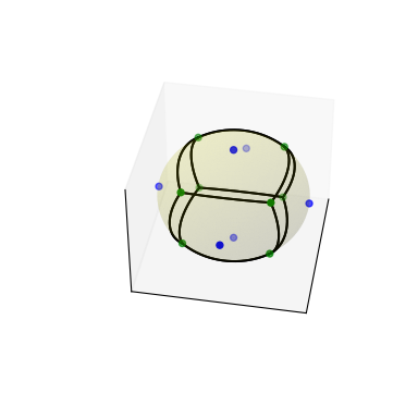
產生繪圖

>>> # sort vertices (optional, helpful for plotting)
>>> sv.sort_vertices_of_regions()
>>> t_vals = np.linspace(0, 1, 2000)
>>> fig = plt.figure()
>>> ax = fig.add_subplot(111, projection='3d')
>>> # plot the unit sphere for reference (optional)
>>> u = np.linspace(0, 2 * np.pi, 100)
>>> v = np.linspace(0, np.pi, 100)
>>> x = np.outer(np.cos(u), np.sin(v))
>>> y = np.outer(np.sin(u), np.sin(v))
>>> z = np.outer(np.ones(np.size(u)), np.cos(v))
>>> ax.plot_surface(x, y, z, color='y', alpha=0.1)
>>> # plot generator points
>>> ax.scatter(points[:, 0], points[:, 1], points[:, 2], c='b')
>>> # plot Voronoi vertices
>>> ax.scatter(sv.vertices[:, 0], sv.vertices[:, 1], sv.vertices[:, 2],
...                    c='g')
>>> # indicate Voronoi regions (as Euclidean polygons)
>>> for region in sv.regions:
...    n = len(region)
...    for i in range(n):
...        start = sv.vertices[region][i]
...        end = sv.vertices[region][(i + 1) % n]
...        result = geometric_slerp(start, end, t_vals)
...        ax.plot(result[..., 0],
...                result[..., 1],
...                result[..., 2],
...                c='k')
>>> ax.azim = 10
>>> ax.elev = 40
>>> _ = ax.set_xticks([])
>>> _ = ax.set_yticks([])
>>> _ = ax.set_zticks([])
>>> fig.set_size_inches(4, 4)
>>> plt.show()

../../_images/scipy-spatial-SphericalVoronoi-1.png

屬性:

points形狀為 (npoints, ndim) 的雙精度陣列: 用於產生 Voronoi 圖的 ndim 維度點
radius雙精度浮點數: 球體半徑
center形狀為 (ndim,) 的雙精度陣列: 球體中心
vertices形狀為 (nvertices, ndim) 的雙精度陣列: 對應於點的 Voronoi 頂點
regions形狀為 (npoints, _ ) 的整數列表的列表: 第 n 個條目是一個列表，其中包含屬於 points 中第 n 個點的頂點索引

方法

calculate_areas()

計算 Voronoi 區域的面積。