scipy.spatial.

HalfspaceIntersection

class scipy.spatial.HalfspaceIntersection(halfspaces, interior_point, incremental=False, qhull_options=None)

N 維空間中的半空間交集。

在 0.19.0 版本中加入。

參數:

halfspacesndarray of floats, shape (nineq, ndim+1)

格式為 [A; b] 的 Ax + b <= 0 形式的堆疊不等式

interior_pointndarray of floats, shape (ndim,)

明顯位於半空間定義區域內部的點。也稱為可行點，可以透過線性規劃獲得。

incrementalbool, optional

允許增量新增半空間。這會佔用一些額外資源。

qhull_optionsstr, optional

傳遞給 Qhull 的額外選項。詳情請參閱 Qhull 手冊。（預設值：ndim > 4 時為 “Qx”，否則為 “”）選項 “H” 始終啟用。

引發:

QhullError

當 Qhull 遇到錯誤情況時引發，例如未啟用解決選項時的幾何退化。

ValueError

如果給定的輸入陣列不相容則引發。

註解

交集是使用 Qhull 函式庫 計算的。這重現了 Qhull 的 “qhalf” 功能。

參考文獻

[Qhull]

http://www.qhull.org/

[1]

S. Boyd, L. Vandenberghe, Convex Optimization，可於 http://stanford.edu/~boyd/cvxbook/ 取得

範例

在您的瀏覽器中試試看！

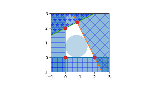
形成某些多邊形的平面的半空間交集

>>> from scipy.spatial import HalfspaceIntersection
>>> import numpy as np
>>> halfspaces = np.array([[-1, 0., 0.],
...                        [0., -1., 0.],
...                        [2., 1., -4.],
...                        [-0.5, 1., -2.]])
>>> feasible_point = np.array([0.5, 0.5])
>>> hs = HalfspaceIntersection(halfspaces, feasible_point)

繪製半空間為填充區域和交點

>>> import matplotlib.pyplot as plt
>>> fig = plt.figure()
>>> ax = fig.add_subplot(1, 1, 1, aspect='equal')
>>> xlim, ylim = (-1, 3), (-1, 3)
>>> ax.set_xlim(xlim)
>>> ax.set_ylim(ylim)
>>> x = np.linspace(-1, 3, 100)
>>> symbols = ['-', '+', 'x', '*']
>>> signs = [0, 0, -1, -1]
>>> fmt = {"color": None, "edgecolor": "b", "alpha": 0.5}
>>> for h, sym, sign in zip(halfspaces, symbols, signs):
...     hlist = h.tolist()
...     fmt["hatch"] = sym
...     if h[1]== 0:
...         ax.axvline(-h[2]/h[0], label='{}x+{}y+{}=0'.format(*hlist))
...         xi = np.linspace(xlim[sign], -h[2]/h[0], 100)
...         ax.fill_between(xi, ylim[0], ylim[1], **fmt)
...     else:
...         ax.plot(x, (-h[2]-h[0]*x)/h[1], label='{}x+{}y+{}=0'.format(*hlist))
...         ax.fill_between(x, (-h[2]-h[0]*x)/h[1], ylim[sign], **fmt)
>>> x, y = zip(*hs.intersections)
>>> ax.plot(x, y, 'o', markersize=8)

預設情況下，qhull 不提供計算內部點的方法。這可以使用線性規劃輕鬆計算。考慮 \(Ax + b \leq 0\) 形式的半空間，求解線性規劃

\[ \begin{align}\begin{aligned}max \: y\\s.t. Ax + y ||A_i|| \leq -b\end{aligned}\end{align} \]

其中 \(A_i\) 是 A 的列，即每個平面的法向量。

將產生一個點 x，該點 x 是凸多面體內最遠的點。準確來說，它是內切於多面體的最大超球體的中心，半徑為 y。此點稱為多面體的 Chebyshev 中心（參見 [1] 4.3.1, pp148-149）。Qhull 輸出的方程式始終是標準化的。

>>> from scipy.optimize import linprog
>>> from matplotlib.patches import Circle
>>> norm_vector = np.reshape(np.linalg.norm(halfspaces[:, :-1], axis=1),
...     (halfspaces.shape[0], 1))
>>> c = np.zeros((halfspaces.shape[1],))
>>> c[-1] = -1
>>> A = np.hstack((halfspaces[:, :-1], norm_vector))
>>> b = - halfspaces[:, -1:]
>>> res = linprog(c, A_ub=A, b_ub=b, bounds=(None, None))
>>> x = res.x[:-1]
>>> y = res.x[-1]
>>> circle = Circle(x, radius=y, alpha=0.3)
>>> ax.add_patch(circle)
>>> plt.legend(bbox_to_anchor=(1.6, 1.0))
>>> plt.show()

返回在新分頁中開啟

屬性:

halfspacesndarray of double, shape (nineq, ndim+1)

輸入半空間。

interior_point :ndarray of floats, shape (ndim,)

輸入內部點。

intersectionsndarray of double, shape (ninter, ndim)

所有半空間的交集。

dual_pointsndarray of double, shape (nineq, ndim)

輸入半空間的對偶點。

dual_facetslist of lists of ints

形成對偶凸包（不一定是單純形）面的點的索引。

dual_verticesndarray of ints, shape (nvertices,)

形成對偶凸包頂點的半空間索引。對於 2-D 凸包，頂點以逆時針順序排列。對於其他維度，它們以輸入順序排列。

dual_equationsndarray of double, shape (nfacet, ndim+1)

[法向量, 偏移量] 形成對偶面的超平面方程式（更多資訊請參閱 Qhull 文件）。

dual_areafloat

對偶凸包的面積

dual_volumefloat

對偶凸包的體積

方法

add_halfspaces(halfspaces[, restart])	處理一組額外的新半空間。
close()	完成增量處理。