scipy.signal.ShortTimeFFT.

頻譜圖

ShortTimeFFT.spectrogram(x, y=None, detr=None, *, p0=None, p1=None, k_offset=0, padding='zeros', axis=-1)

計算頻譜圖或交叉頻譜圖。

頻譜圖是 STFT 的絕對值平方，亦即對於給定的 S[q,p]，其值為 abs(S[q,p])**2，因此始終為非負值。對於兩個 STFT Sx[q,p]、Sy[q,p]，交叉頻譜圖定義為 Sx[q,p] * np.conj(Sy[q,p])，且為複數值。這是一個方便的函式，用於呼叫 stft / stft_detrend，因此所有參數都在那裡討論。如果 y 不是 None，則它需要與 x 具有相同的形狀。

另請參閱

stft

執行短時傅立葉轉換。

stft_detrend

STFT，從每個區段中減去趨勢。

scipy.signal.ShortTimeFFT

此方法所屬的類別。

範例

在您的瀏覽器中試試看！

以下範例顯示一個頻率變化的方波頻譜圖 \(f_i(t)\) (在圖中以綠色虛線標記)，以 20 Hz 採樣

>>> import matplotlib.pyplot as plt
>>> import numpy as np
>>> from scipy.signal import square, ShortTimeFFT
>>> from scipy.signal.windows import gaussian
...
>>> T_x, N = 1 / 20, 1000  # 20 Hz sampling rate for 50 s signal
>>> t_x = np.arange(N) * T_x  # time indexes for signal
>>> f_i = 5e-3*(t_x - t_x[N // 3])**2 + 1  # varying frequency
>>> x = square(2*np.pi*np.cumsum(f_i)*T_x)  # the signal

使用的 Gaussian 視窗為 50 個樣本或 2.5 秒長。參數 mfft=800 (過採樣因子 16) 和 hop 間隔 2 在 ShortTimeFFT 中被選擇來產生足夠的點數

>>> g_std = 12  # standard deviation for Gaussian window in samples
>>> win = gaussian(50, std=g_std, sym=True)  # symmetric Gaussian wind.
>>> SFT = ShortTimeFFT(win, hop=2, fs=1/T_x, mfft=800, scale_to='psd')
>>> Sx2 = SFT.spectrogram(x)  # calculate absolute square of STFT

圖表的色圖以對數方式縮放，因為功率譜密度以 dB 為單位。訊號 x 的時間範圍以垂直虛線標記，陰影區域標記邊界效應的存在

>>> fig1, ax1 = plt.subplots(figsize=(6., 4.))  # enlarge plot a bit
>>> t_lo, t_hi = SFT.extent(N)[:2]  # time range of plot
>>> ax1.set_title(rf"Spectrogram ({SFT.m_num*SFT.T:g}$\,s$ Gaussian " +
...               rf"window, $\sigma_t={g_std*SFT.T:g}\,$s)")
>>> ax1.set(xlabel=f"Time $t$ in seconds ({SFT.p_num(N)} slices, " +
...                rf"$\Delta t = {SFT.delta_t:g}\,$s)",
...         ylabel=f"Freq. $f$ in Hz ({SFT.f_pts} bins, " +
...                rf"$\Delta f = {SFT.delta_f:g}\,$Hz)",
...         xlim=(t_lo, t_hi))
>>> Sx_dB = 10 * np.log10(np.fmax(Sx2, 1e-4))  # limit range to -40 dB
>>> im1 = ax1.imshow(Sx_dB, origin='lower', aspect='auto',
...                  extent=SFT.extent(N), cmap='magma')
>>> ax1.plot(t_x, f_i, 'g--', alpha=.5, label='$f_i(t)$')
>>> fig1.colorbar(im1, label='Power Spectral Density ' +
...                          r"$20\,\log_{10}|S_x(t, f)|$ in dB")
...
>>> # Shade areas where window slices stick out to the side:
>>> for t0_, t1_ in [(t_lo, SFT.lower_border_end[0] * SFT.T),
...                  (SFT.upper_border_begin(N)[0] * SFT.T, t_hi)]:
...     ax1.axvspan(t0_, t1_, color='w', linewidth=0, alpha=.3)
>>> for t_ in [0, N * SFT.T]:  # mark signal borders with vertical line
...     ax1.axvline(t_, color='c', linestyle='--', alpha=0.5)
>>> ax1.legend()
>>> fig1.tight_layout()
>>> plt.show()

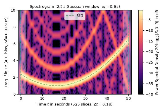
對數縮放揭示了方波的奇次諧波，這些諧波在 10 Hz 的奈奎斯特頻率處被反射。這種混疊也是圖中雜訊偽影的主要來源。

返回在新分頁中開啟