gaussian_filter#
- scipy.ndimage.gaussian_filter(input, sigma, order=0, output=None, mode='reflect', cval=0.0, truncate=4.0, *, radius=None, axes=None)[source]#
多維高斯濾波器。
- 參數:
- inputarray_like
輸入陣列。
- sigma純量或純量序列
高斯核心的標準差。高斯濾波器的標準差是針對每個軸以序列或單一數字給出,在單一數字的情況下,所有軸都相等。
- orderint 或 int 序列,選用
沿每個軸的濾波器階數以整數序列或單一數字給出。階數 0 對應於與高斯核心的卷積。正階數對應於與高斯導數的卷積。
- output陣列或 dtype,選用
放置輸出的陣列,或返回陣列的 dtype。預設情況下,將建立與輸入相同 dtype 的陣列。
- modestr 或 序列,選用
mode 參數決定當濾波器重疊邊界時,輸入陣列如何延伸。透過傳遞模式序列,其長度等於輸入陣列的維度數量,可以沿每個軸指定不同的模式。預設值為 ‘reflect’。有效值及其行為如下
- ‘reflect’ (d c b a | a b c d | d c b a)
輸入透過反射最後一個像素的邊緣來延伸。此模式有時也稱為半樣本對稱。
- ‘constant’ (k k k k | a b c d | k k k k)
輸入透過以相同的常數值填充邊緣之外的所有值來延伸,常數值由 cval 參數定義。
- ‘nearest’ (a a a a | a b c d | d d d d)
輸入透過複製最後一個像素來延伸。
- ‘mirror’ (d c b | a b c d | c b a)
輸入透過反射最後一個像素的中心來延伸。此模式有時也稱為全樣本對稱。
- ‘wrap’ (a b c d | a b c d | a b c d)
輸入透過環繞到相對邊緣來延伸。
為了與內插函數保持一致,也可以使用以下模式名稱
- ‘grid-constant’
這是 ‘constant’ 的同義詞。
- ‘grid-mirror’
這是 ‘reflect’ 的同義詞。
- ‘grid-wrap’
這是 ‘wrap’ 的同義詞。
- cval純量,選用
如果 mode 為 ‘constant’,則填充輸入邊緣之外的值。預設值為 0.0。
- truncatefloat,選用
在此標準差數量處截斷濾波器。預設值為 4.0。
- radiusNone 或 int 或 int 序列,選用
高斯核心的半徑。半徑是針對每個軸以序列或單一數字給出,在單一數字的情況下,所有軸都相等。如果指定,則沿每個軸的核心大小將為
2*radius + 1,並且 truncate 會被忽略。預設值為 None。- axesint 或 None 的元組,選用
如果為 None,則沿所有軸篩選 input。否則,沿指定的軸篩選 input。當指定 axes 時,用於 sigma、order、mode 和/或 radius 的任何元組都必須符合 axes 的長度。這些元組中的第 i 個條目對應於 axes 中的第 i 個條目。
- 返回:
- gaussian_filterndarray
返回與 input 相同形狀的陣列。
註解
多維濾波器實作為 1-D 卷積濾波器序列。中間陣列以與輸出相同的資料類型儲存。因此,對於精度有限的輸出類型,結果可能不精確,因為中間結果可能以不夠的精度儲存。
高斯核心沿每個軸的大小將為
2*radius + 1。如果 radius 為 None,則將使用預設的radius = round(truncate * sigma)。範例
>>> from scipy.ndimage import gaussian_filter
>>> import numpy as np
>>> a = np.arange(50, step=2).reshape((5,5))
>>> a
array([[ 0,  2,  4,  6,  8],
       [10, 12, 14, 16, 18],
       [20, 22, 24, 26, 28],
       [30, 32, 34, 36, 38],
       [40, 42, 44, 46, 48]])
>>> gaussian_filter(a, sigma=1)
array([[ 4,  6,  8,  9, 11],
       [10, 12, 14, 15, 17],
       [20, 22, 24, 25, 27],
       [29, 31, 33, 34, 36],
       [35, 37, 39, 40, 42]])
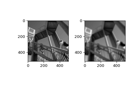
>>> from scipy import datasets
>>> import matplotlib.pyplot as plt
>>> fig = plt.figure()
>>> plt.gray()  # show the filtered result in grayscale
>>> ax1 = fig.add_subplot(121)  # left side
>>> ax2 = fig.add_subplot(122)  # right side
>>> ascent = datasets.ascent()
>>> result = gaussian_filter(ascent, sigma=5)
>>> ax1.imshow(ascent)
>>> ax2.imshow(result)
>>> plt.show()