scipy.interpolate.RectSphereBivariateSpline.

__call__

RectSphereBivariateSpline.__call__(theta, phi, dtheta=0, dphi=0, grid=True)

在給定位置評估樣條函數或其導數。

參數:

theta, phiarray_like（類陣列）

輸入座標。

如果 grid 為 False，則在點 (theta[i], phi[i]), i=0, ..., len(x)-1 評估樣條函數。 遵循標準 Numpy 廣播規則。

如果 grid 為 True：在由座標陣列 theta, phi 定義的網格點上評估樣條函數。 陣列必須按遞增順序排序。 軸的順序與 np.meshgrid(..., indexing="ij") 一致，且與預設順序 np.meshgrid(..., indexing="xy") 不一致。

dthetaint，選填

theta 導數的階數

在版本 0.14.0 中新增。

dphiint

phi 導數的階數

在版本 0.14.0 中新增。

gridbool

是否要在輸入陣列所跨越的網格上評估結果，或在輸入陣列指定的點上評估結果。

在版本 0.14.0 中新增。

範例

在您的瀏覽器中試試看！

假設我們想要使用樣條函數在球面上內插一個雙變數函數。 該函數的值在經度和緯度的網格上已知。

>>> import numpy as np
>>> from scipy.interpolate import RectSphereBivariateSpline
>>> def f(theta, phi):
...     return np.sin(theta) * np.cos(phi)

我們在網格上評估該函數。 請注意，meshgrid 的預設 indexing="xy" 會在內插後產生非預期的（轉置）結果。

>>> thetaarr = np.linspace(0, np.pi, 22)[1:-1]
>>> phiarr = np.linspace(0, 2 * np.pi, 21)[:-1]
>>> thetagrid, phigrid = np.meshgrid(thetaarr, phiarr, indexing="ij")
>>> zdata = f(thetagrid, phigrid)

接下來，我們設定內插器並使用它在更精細的網格上評估該函數。

>>> rsbs = RectSphereBivariateSpline(thetaarr, phiarr, zdata)
>>> thetaarr_fine = np.linspace(0, np.pi, 200)
>>> phiarr_fine = np.linspace(0, 2 * np.pi, 200)
>>> zdata_fine = rsbs(thetaarr_fine, phiarr_fine)

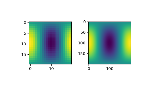
最後，我們將粗略採樣的輸入資料與精細採樣的內插資料一起繪製，以檢查它們是否一致。

>>> import matplotlib.pyplot as plt
>>> fig = plt.figure()
>>> ax1 = fig.add_subplot(1, 2, 1)
>>> ax2 = fig.add_subplot(1, 2, 2)
>>> ax1.imshow(zdata)
>>> ax2.imshow(zdata_fine)
>>> plt.show()

返回在新分頁中開啟